MANAGING COMMON AND EXPECTED UNCERTAINTY IN DISTRIBUTION

Critical Strategic Information to Extend the TOC Replenishment Solution

Eli Schragenheim and Michael Demere

Executive Summary

This paper is written mainly for distribution to retail. Much of it applies to other kinds of distribution as well, and the text says where it applies fully and where only in part.

The central problem in managing any supply chain is uncertainty. Demand varies, supply varies, and the organization’s own internal variation adds to the difficulty of serving its customers reliably.

In retail the problem shows most clearly in the long tail: thousands of slow-moving items that tie up cash and shelf space and drag down the return on the inventory investment. Trimmed one sensible cut at a time, the tail slowly hollows out the very assortment customers come for. The usual tools offer no way out: the tail cannot be forecast, and stocking all of it cannot be afforded. So most distributors manage it by reflex, and lose ground they never see leaving.

The tail is a problem of uncertainty, and managing it significantly better is the single subject of this paper. Not forecasting it away, and not merchandising around it: how to manage the common recurring variation in demand and supply that every distributor lives with, item by item across the whole catalog.

There is a better way, and it is already well known. Eli Goldratt often observed that the TOC Replenishment Solution is the most powerful application of the Theory of Constraints, and yet the least implemented.

The question remains: why?

The solution itself is simple: hold inventory at the point of highest aggregation, and replenish frequently from actual consumption. Where implemented, the results are dramatic (better availability, less inventory, stronger cash flow), as Goldratt’s Isn’t It Obvious? demonstrates.

Yet the basic principles leave one practical question unanswered: protecting every SKU (Stock Keeping Unit) to the same degree is not economical, so a distributor needs a clear strategy for how hard to commit to each item, and the practical options that follow from that choice.

The real power of the Replenishment Solution is wider. It becomes complete the moment a distributor stops treating full availability as the default and starts choosing, deliberately and item by item, how much availability to commit to. The unlocking idea is simple and slightly uncomfortable: a stockout is not always a lost sale. When that is true, full availability becomes one option among three, and the solution reaches the entire catalog, tail included.

Several of the decisions this paper develops are, in the classical sense, marketing strategy: who is being served, what assortment serves them, how deeply to commit to categories and items. The paper treats them as strategic information because they sit upstream of replenishment: marketing as segmentation, assortment, and stock levels, not as advertising or promotion.

We arrived at the answer through direct observation. The Replenishment Solution works beautifully for fast- and medium-moving items with reliable supply. Extended to the long tail, or to unreliable supply, the inventory required to protect availability looked unreasonably high. Rather than accept the limitation, we asked: what would a complete, practical solution look like?

The answer starts where distributors already live: with uncertainty. Demand and supply vary, and that variation is not a forecasting failure waiting for better technology to fix. A forecast is a range, not a number. The practical response is a decision, made item by item, about how much availability is worth committing to, and the replenishment discipline to deliver it.

Two contributions make that possible.

Both rest on correcting one costly assumption: that a stockout is always a lost sale. Usually it is not, and once that is recognized, committing less than full availability for some items becomes sound strategy rather than failure.

The first is the recognition that not every item warrants the same commitment. Three named strategies make the choice explicit.

  • Assured Availability commits to having the item in stock whenever a customer wants it, operationally close to perfect, for items where that commitment is justified.
  • Reasonable Availability aims for the item to be usually available, accepting occasional stockouts as part of the deal.
  • Limited Availability carries the item selectively, with no standing commitment, appropriate where surplus inventory itself poses real financial risk.

The error is not in choosing a less-than-perfect strategy for some items; it is in failing to choose deliberately.

That choice is made systematically rather than by instinct. For every item, four sequenced decisions are in play, with one prior question: what is the customer actually shopping for? First, should the item be sold at all? Some items do not earn their place. Second, if yes, should we invest to make availability perfect or near-perfect? That is Assured Availability. Third, if not, what level are we aiming for? That is the territory of Reasonable Availability, which is valid especially when the customer can easily buy another product instead. Fourth, where surplus inventory itself poses financial risk, how much do we keep of only what we are confident will sell before the value evaporates? That is Limited Availability. Every item falls into one of these four answers, and the contribution is making the choice deliberate rather than implicit.

These choices cannot be made in a vacuum. They depend on knowing whom the distributor serves, what it commits to delivering, and what its supply and finances can sustain. Without that context, decisions are made inconsistently, and individually reasonable decisions aggregate into strategic incoherence.

The second is that the commitment need not be made to an individual item at all. What the customer is shopping for decides where availability should be promised. Someone who wants Glenfiddich wants that bottle; someone who wants salt will take any of several; someone who wants a pair of jeans has come to choose from a range. Availability can therefore be committed at the level of a set: a Like Product Group, where one available member satisfies the need, or a whole assortment, where what must be protected is the richness of the choice itself. Buffers then work in two layers: items that the strategy wants to keep selling have their own buffer, while the set is held to a commitment of its own, and the set’s protection is the number of members it can offer. Many tail items that could never justify a standing commitment alone earn their place comfortably inside a set that offers a choice.

The stakes are significant. The long tail often represents half or more of a distributor’s SKU count while contributing a small share of revenue. Managed poorly, it consumes working capital, space, and attention. Managed well, it differentiates: it serves valuable segments, offers variety, and opens the way for new products and new tastes, completing the offering that drives loyalty.

Not all of this is new, and the paper is careful about which parts are. Much of the machinery (the Replenishment Solution itself, buffer management, the throughput frame) is established TOC, and the paper uses it as such. Three things are new, each filling a gap the established solution left open: the three availability strategies and the reasoning beneath them; two-layer buffering, which commits availability to a set rather than to an individual item; and the assortment managed as a counting buffer of variety. The body develops why each goes beyond what the Replenishment Solution already provided.

Distribution has always lived with this uncertainty. Managed deliberately rather than forecast away, it becomes an advantage few competitors capture.

The Key Challenge in Distribution

Managing the Common and Expected Uncertainty

The role of a distribution organization is to bridge what customers want to buy and what suppliers can provide, with both sides subject to considerable uncertainty. Most of the time the distributor has to guess the demand for specific products, taking supply time into account, while both demand and supply time fluctuate constantly. Managing this gap for thousands of items across many stores, where the demand for every item at every store has to be managed, is a real challenge.

Online shopping relaxes the challenge a little, but it makes customers wait, moving part of the uncertainty onto them. The need to purchase goods almost immediately still makes physical stores necessary.

The key tool in supply chains is forecasting. Whether produced by algorithms, AI, or human estimation, the forecast states what demand is going to be, so quantitative decisions can be made.

Yet one-number forecasts are unreliable even before considering rare events like a war closing supply routes. Common and expected uncertainty looks only at the normal, ongoing small happenings with non-dramatic impact on customer preferences, supply time, and product quality. Its defining trait: sometimes the different fluctuations accumulate, and at other times they cancel each other out. 

Managing the common and expected uncertainty is a serious challenge, disrupting the bridge between demand and supply. And this is where the real opportunity lies: significantly better service than the competition, without taking high risks.

None of this criticizes how distributors have managed until now. Uncertainty is hard, and the goal is to give it a name and a structure. A distributor that recognizes it openly, judging a decision by the uncertainty it faced rather than by how it turned out and managing it more carefully than its competitors, turns what everyone lives with into a real advantage.

Where This Paper Applies

This paper uses distribution in its broad sense: buying goods and making them available to whoever needs them, without changing the product. A retail chain is a distributor under that definition. So is an industrial supply house, a pharmacy, a spare-parts operation and a wholesaler serving manufacturers. The paper is written mainly for distribution to retail, where the number of item-locations makes the uncertainty hardest to manage, but most of it applies wherever goods are bought in order to be sold again.

Within that definition, readers will recognize themselves in one of two situations, and the difference needs to be named at the start.

In the first, the customer chooses. Someone shopping for a hat, a book or a bottle of wine has a need that several products would satisfy, and part of what that customer is buying is the choice itself. A distributor serving that customer has to decide what variety to carry, and the risk of being short is that the customer finds nothing appealing.

In the second, the customer has already chosen. A manufacturer that has qualified one compressor for its refrigerator will not accept a different one. A contractor who has standardized on a particular carton sealing tape wants that tape, not an identical tape from another maker. Here there is no selection to manage. The distributor’s task is to have the specific item when it is asked for, and the risk of being short is that the customer is not served at all.

Most distributors live in both situations at once, in different proportions. A grocery chain is mostly the first, an industrial supply house mostly the second, and each has some of the other. The proportion decides which chapters carry the most weight for a given reader. Reasonable Availability, for instance, is typical of retail and rarer elsewhere; the chapters on Like Product Groups and assortments matter most where customers substitute.

What does not change with the proportion is the set of decisions that has to be made. In both situations demand and supply vary in ways no forecast removes. In both, someone has to decide how much stock to hold against that variation and what holding it is worth against what the item returns. In both, availability is a promise to the customer, and promising full availability on everything costs enough that it deserves to be a decision rather than a habit. Where a chapter applies only partially outside retail, the text says so at the point it happens.

What This Paper Does Not Cover

This approach applies mainly to distribution strategies that intend to replenish the items they sell, not to strategies where a sold product is never reordered. Two familiar examples make the boundary concrete. Some fashion retailers, Zara being the best known, buy a design once, sell it, and move on. Certain fresh fruits and vegetables behave the same way: available for a short window, then replaced by something else. Nothing here judges those strategies; they are simply built on a different premise.

The boundary is structural. Every mechanism in these pages (the stock buffer, buffer management, replenishing to consumption) presupposes the stock-buffer can be restored. Where there is no intention to reorder, there is no buffer to manage: the decision is a one-time purchase, not an ongoing commitment to availability.

Such strategies fall outside the item layer only. A retailer who never replenishes a particular garment still manages the richness of what hangs on the rack, refreshing it constantly with different items. That is a commitment at the level of the assortment, and the chapters on Like Product Groups and Managing Assortments apply to it directly.

The paper also sets aside several decisions that matter to a distributor but sit outside the question of uncertainty. It does not address the classification of an assortment by depth or breadth, or the life-cycle of an item, meaning when a product is emerging, at its peak, or reaching the end of its life. It does not address market segmentation, the choice of which customers to serve. And it does not offer a method for deciding which items belong in the catalog at all, or when a dead item, one that has lost its demand and will not regain it, should be dropped; the paper takes as given that such decisions must be made, and leaves the making of them to the people close to the market. These are real and important disciplines, and they are the established expertise of merchandisers and category managers, who generally know how to handle them. What that expertise does not resolve is how to manage the common and expected uncertainty around whatever assortment results. That, and only that, is the subject of this paper.

Forecasts Are Ranges

The real challenge in supply chain management is not how to forecast better; it is how to manage uncertainty. Uncertainty is a fact; a better forecast reduces it a little, but it does not go away. Many executives now expect AI to solve the problem, and AI is delivering improvements in inventory accuracy, supplier analytics, and short-horizon demand sensing. Those gains are real. But when AI is applied to forecasting while the logic still produces a single number, we are optimizing a flawed approach rather than fixing it. A single number gives no sense of how far actual demand might reasonably deviate from it, and that is exactly the information needed to decide how much to stock. A more sophisticated single number is still a single number. The ceiling on that kind of improvement is low. The limit is in the paradigm, not the math: until common and expected uncertainty is addressed, even the most advanced AI-assisted forecast gives a better wrong answer, not a different kind of answer.

We are largely blind to this. Organizations treat the forecast as if it were the demand rather than an estimated average of it. Plans are built on the number; performance is measured against it. When actual demand comes in different, the reaction is to question the forecaster, not the assumption that a single number was ever appropriate.

The mistake is easily demonstrated. A sales team forecasts demand for an item next month at 1,200 units; the supply chain system treats 1,200 as the plan; operations stocks accordingly. Actual demand might have been 798 or 1,426. The forecast was not wrong; 1,200 was only the average of a range that would have read 750–1,650. And since only 1,200 were stocked and all were sold, the higher demand was never even recorded. A specific number looks authoritative, and it is almost always wrong. The forecasting team did not do a bad job; the thing being forecast is not a number. It is a range.

Eli Goldratt made this point repeatedly and forcefully. A forecast, properly understood, describes the highest likelihood in a band of possible outcomes. The actual demand will fall somewhere inside that band, and the organization’s job is to be ready to respond wherever inside the band it falls, rather than to predict the spot.

The range has a shape that matters. The further from actual consumption, the wider the Forecast Range: a forecast for a week twelve months out is a wide band; for next week, a narrower one. That shape is a feature of how demand behaves, not a limitation of forecasting technology. The narrowing is not strictly monotonic: tomorrow’s band can be wider than the coming week’s, because daily fluctuations average out over a few days. Within any window, the relevant uncertainty depends on how the variation aggregates.

This is why response time matters so much. An organization that reacts quickly to actual consumption operates inside the narrow part of the Forecast Range, where uncertainty is containable. One that commits to a single-number plan far in advance operates in the wide part, where the commitment cannot match what materializes. Better forecasting does not close that gap; faster response does.

This raises the question of the forecasting horizon. A three-month forecast may seem more reliable than a two-week one. But when the reliable supply time is two weeks, replenishing what was sold is the right response to the actual uncertainty, and the three-month forecast serves no decision that has to be taken today.

Understanding uncertainty therefore means resisting the single-number forecast and working with the Forecast Range, with a horizon that matches the response time. The question changes from “what number will demand be?” to “what range is demand likely to fall within, and how quickly can we respond to wherever it lands?” This reframe is what makes the rest of the argument in this paper possible.

The effective way to handle uncertainty is to recognize it openly, understand the possible outcomes, and outline the rational options. No decision should be judged without understanding the uncertainty the decision maker faced. The gain is reaching new levels of success by handling uncertainty more effectively than the competition.

The Uncertainty That Cannot Be Solved

Organizations often approach future demand, most notably for the long tail, as a problem to be solved: better forecasting, more sophisticated algorithms, on the implicit assumption that enough data and analytical power can reduce uncertainty to acceptable levels.

The assumption is false for all items, and more so for tail items. The uncertainty is not a temporary condition to be overcome; it is a permanent feature of sparse demand. No analytical sophistication will tell you whether the specialty component that sold twice last quarter will sell three times next quarter or zero. The data does not contain that answer.

Acknowledging this changes the problem. The question is not “how do we predict demand for a specific item in a specific location?” but “how do we make good ordering decisions, especially for tail items, despite irreducible uncertainty?” Organizations that pursue prediction accuracy waste resources on an impossible objective; organizations that accept uncertainty and build decision frameworks around it make progress.

The Key Elements of the TOC Replenishment Solution

This paper expands the TOC application for distribution companies.  Here we summarize the key elements behind the application.

The most important element is the stock buffer. The name already points to its role: protecting the availability of an item from fluctuations in both demand and supply. The buffer is defined for every item offered for sale, and it includes the on-hand stock available for sale plus the stock still on the way, including orders the supplier has not yet shipped.

The stock buffer is kept constant unless a clear decision is made to change its size, either because it fails too often to protect availability, or because too much of it sits on-hand for too long, meaning the buffer is too high.

Because the stock buffer is kept constant, every sale must be replenished as fast as possible. Usually, each day’s sales per item are accumulated and a replenishment request for that quantity is issued, keeping the buffer intact. The buffer operates like the ‘Min’ in the Min-Max practice: whenever the stock plus already-issued replenishment orders fall below the Min, a new order is generated. TOC recommends replenishing only up to the Min, the buffer size, without a minimum batch. Sometimes reality forces a minimum batch, but its necessity should always be checked.

Another key element is Buffer Management: ongoing control of the on-hand stock. While the stock buffer is kept constant, the on-hand part goes down with every sale and up again when replenishment arrives. Its purpose is to quickly note the cases where on-hand stock is so low that a shortage is imminent unless the replenishment arrives fast.

Buffer Management looks at the ratio ((Stock Buffer minus On-Hand) × 100 / Stock Buffer), the penetration into the buffer, or how much of it is not on-hand. This is the buffer status, measured for every item and location every day. Above 67%, with more than two-thirds of the buffer missing, the status is Red. At 33% or less the status is Green: a safe situation, maybe too safe. Between them the status is Yellow.

Operationally we expect to try to expedite the Red replenishment orders, in order to prevent shortages.  

For a distribution chain, a key element is the prominent role of the central warehouse: much more inventory at the center, and fast replenishment from the center to the stores. Every store can then hold relatively small buffers, because its replenishment time is very short.

The central warehouse is replenished by suppliers, whose response is usually slower than the warehouse’s own replenishment of the stores or other downstream locations. But because the center covers the demand and supply uncertainty of the whole network, its accumulated demand fluctuates far less than the demand at any single store. Dealing with all the suppliers at the center, and feeding all the stores from actual sales, is what makes the common and expected uncertainty manageable.

This paper recognizes the huge power of the above solution, but also some situations where certain deviations should be used.  On the way, we highlight the main challenge all supply-chains, definitely all distribution organizations, have to deal with.

Another key TOC term is throughput, similar to the accounting term ‘contribution’: the selling price minus the truly variable costs. For most distributors this is the margin: selling price minus the supplier’s price. In manufacturing and services the ‘margin’ is often reduced by other costs such as transportation, storage, and manpower; in TOC all not-truly-variable costs go into Operating Expenses, and net profit before tax is total throughput minus operating expenses.

A word about independence. Every aggregation in this approach, whether a central warehouse serving many locations or a Like Product Group serving one need, is protected by partial independence: what is short here is usually not short there at the same time. Full independence does not exist in real life, and neither does full dependence; the degree cannot be calculated and there is no need to try. Some dependency simply means somewhat less protection; how much, experience will show.

Three Groups of Products

For this conversation we will classify the potential set of products into three groups: the Fat Top, the Lessening Middle, and the Skinny Tail. This is a classification by how demand behaves, meaning how much and how steadily each item sells, not by revenue, by margin, or by the item’s stage of life, and it is distinct from the availability strategies introduced later.

These groups are not just points on a sales curve; they behave differently because the uncertainty behaves differently. The Fat Top sells fast and steadily, so demand averages out over each short replenishment cycle; the Skinny Tail sells rarely and erratically, so that averaging never happens and every unit of stock carries far more uncertainty per sale. That is why one availability rule cannot serve all three.
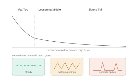
Figure 1. The three product groups along the demand curve, with the demand pattern typical of each.

The three groups might remind readers of ABC analysis, which allocates management attention across items. The difference is basic: the groups point to characteristics that should shape the inventory strategy, as developed later in this paper, while attention priorities in TOC are handled by Buffer Management: the computerized system manages every item from the most recent data plus the key strategy rules.

Others in the field describe a similar split under different labels; head, body, and tail are common. We use the more descriptive Fat Top, Lessening Middle, and Skinny Tail because the names point to the demand-and-supply behavior that drives the inventory strategy, rather than to position on a sales curve alone.

The Fat Top demonstrates the characteristics of high, regular “enough” consumption and certain “enough” replenishment of supply. These are the items where distributors, and also their suppliers, have a high desire to provide excellent ongoing availability, since a lost sale at the shelf is usually a lost sale for the supplier too. We should expect exceptionally high inventory turns: 25+ inventory turns should be a regular expectation.

Every competitor carries the same fast movers, and the resulting competition drives their per-unit throughput to the lowest in the assortment, sometimes to loss-leader levels. The Fat Top is therefore where a distributor is least differentiated; its value is stability, not competitive advantage. The possibilities to excel are much greater in the Lessening Middle.

The challenge begins with the Lessening Middle, where uncertainty in demand and resupply grows. These are items your customers demonstrably want, but with enough uncertainty to produce stockouts or periods of excess. The group is critical: its average margin per unit is usually higher than the Fat Top’s, where competition is fierce, and market shifts move demand sharply up for some members and down for others. The full bottom-line impact of this group is crucial, and the TOC practice of keeping excellent availability of every member while preventing excess inventory makes a true difference to profitability.

The greatest challenge is the Skinny Tail, including the decision which of these items to keep selling, and whether to keep them available at all. It is the hardest group to manage: providing availability for a Skinny Tail item means holding relatively high stock and waiting a long time for it to deplete. Yet these are the products that enrich the choice and attract customers, and losing those customers can be disastrous. So, some form of availability for slow movers is needed.

Demand for these items can be spiky and unpredictable, and vendor replenishment times are often unreliable, which makes any form of assured availability difficult and expensive. It is therefore common for distributors to abandon too many Skinny Tail products, sacrificing revenue even where customers want the items or the wider choice. Worse, every abandoned item is an opening for a competitor to gain a foothold.

The Skinny Tail sits at the heart of a chronic internal argument. Marketing advocates broad choice, more variety and more niche items, hoping to attract customers who would otherwise go elsewhere. Operations and finance push back on carrying cost, space, and working capital.

What is missing from this recurring conversation are two questions that would resolve it: for each Skinny Tail item, is it truly important to some customers, and if so, how much availability does it warrant?

Within the Skinny Tail items, we find items with truly erratic supply or short shelf life, where surplus must be scrapped at real cost. Such items are better handled selectively: carried without surplus rather than under a standing availability commitment.

The groups also differ in where the financial opportunity lives. The Fat Top consists of fast movers with consistent demand, which also makes it the most competitive group, with the lowest per-unit throughput (selling price minus truly variable cost). Its important characteristic is that it is the stable part of the whole business.

The Lessening Middle, by contrast, is where volume multiplied by per-unit throughput can be substantial. Managed well, the Lessening Middle is the group that produces the largest contribution opportunity, and for that reason it is, in many distributors, the most important group in the portfolio. It also calls for considerable management attention to keep excellent availability.

The Three Strategies for Availability

These strategies are a different axis from the three-group classification of Fat Top, Lessening Middle, and Skinny Tail. The groups are descriptive: they describe how an item behaves. The strategies are prescriptive: they describe what the distributor commits to. An item’s group does not dictate its strategy, and the two should not be conflated.

The three strategies are described here in retail terms. For a specialized distributor whose customers do not substitute, Reasonable Availability is rare and the choice is mostly between Assured and Limited; the reasoning is the same.

A simple and seemingly trivial assumption underlies most thinking about availability: what is not on the shelf cannot be sold, and one step further, any shortage causes a loss of sales. The logic is so widely accepted that it rarely gets examined, and it drives organizations toward an implicit goal of perfect availability across the entire assortment. Availability is a decision, not a default.

The logic is only partially true. Items that have already lost their demand do not reduce sales when short; they were not going to sell anyway. For items that do have demand, a stockout is a signal that a sale may have been lost, not evidence that one was. The customer who finds an empty shelf may keep a private buffer at home, take a substitute and think nothing of it, come back next visit, or leave disappointed and never return. The actual damage runs from zero to losing the customer and everything else they would have bought, and there is no clear way to measure where on that range any specific stockout fell. Stockout rates are measurable; the lost sales they produced are not.

This distinction carries the rest of the argument. If every stockout were a lost sale, the only rational strategy would be perfect availability, call it Assured Availability, for every item. Because most stockouts do not lose all the sales, the strategy dilemma is real. Some items earn the cost of Assured Availability because the customer-loss is severe enough to justify it: the rare customer who walks out for good carries more downside than the standing buffer costs. Others live comfortably under Reasonable Availability, available most of the time, because the typical response to an occasional stockout is substitution, deferral, or indifference. Still others belong under Limited Availability, holding little or no surplus, especially items with short expiration, where the customer understands and lives with it.

How critical is excellent availability across the assortment, then? Posed honestly, the question turns on two variables: the cost of providing excellent availability for the specific item, and whether the assortment offers natural substitutes, so that the customer would not be too disappointed by that item’s absence.

Before those decisions can be answered, a prior question has to be settled, because it determines what is being committed to in the first place: what is the customer actually shopping for?

Three answers cover most of what a distributor carries. Some customers come for a specific item, and nothing else will do; the shopper who wants Coca Cola Zero wants that particular item. Some come for a need that any of several items would satisfy, and are indifferent among them, as most customers are about salt. And some come to choose: the shopper looking for a nice hand watch expects to be presented with a range and to pick from it, and would be puzzled by the suggestion that one particular watch was the object of the trip.

The distinction matters because it moves what is being committed. For the first, the commitment is to the item, and the four decisions below apply directly. For the second, it is to the group, the subject of Like Product Groups. For the third, it is to the richness of the choice, the subject of Managing Assortments. Only in the first case is a specific SKU (Stock Keeping Unit) what the distributor is promising. Deciding which applies precedes all the other decisions, and like the tests that follow, it is a judgment made by people close to the customers, not a property of the product category. A particular single-origin coffee is a specific-item purchase for the enthusiast who wants exactly that roast, and an indifferent choice for the host who just wants a decent cup for guests.

The strategic frame can be made explicit. For every item the distributor might carry, four sequenced decisions are in play:

  1. Should the item be sold at all?
  2. If yes, should we make the full investment to ensure availability is perfect or near-perfect? If so, the item belongs under Assured Availability, and the rest of the approach (buffers, replenishment, governance) is tuned accordingly.
  3. If perfect availability is not warranted, what level of availability are we aiming for? This is the territory of Reasonable Availability, where the item is available at a level chosen to be good enough for its role, accepting that some stockouts come with it.
  4. For items where surplus inventory itself poses a financial risk (short expiration, obsolescence, items where being wrong on the upside dwarfs being wrong on the downside), how much do we keep of only what we are certain will sell before the value evaporates? This is Limited Availability.

Assured Availability demands holding considerably more inventory than the average forecast predicts, considering also the reliable supply time, and even expediting when demand is high and regular supply is slow.

Reasonable is much less demanding, still ongoing control is required to ensure good enough availability.

Limited Availability tries to prevent too high stock.  Thus, while availability is still desired, the message to the customers is: “when you see, grab it.”

How the Item-Strategies Map to the Three Groups

The three item strategies are not a renaming of the Fat Top, Lessening Middle, and Skinny Tail. The product groups are descriptive: they characterize the demand and supply behavior of items. The strategies are prescriptive: they describe what the distributor commits to do about availability. The mapping between them is real but loose and the looseness matters.

The Fat Top, by definition, has steady demand and responsive supply: almost every Fat Top item belongs under Assured Availability, and the volume justifies the buffer. Lessening Middle items split: those with strong enough demand and tolerable supply earn the assured commitment, while the more variable ones are better served by Reasonable Availability than by over-investing. The Skinny Tail, meaning only those items the strategy wants to keep selling, splits between very few Assured, mainly Reasonable, and some Limited Availability. Strategically important items that signal expertise to priority customers may earn Assured Availability despite low velocity; items dominated by expiration or obsolescence risk belong under Limited Availability, where the carrying cost is honest about its bound; the rest, worth offering but not critical, belong under Reasonable Availability.

Two qualifications matter for how this gets applied.

The first is that the choice is per item, not per group. Two Skinny Tail items may receive opposite strategies because their strategic role differs. 

The second is that new products default to Reasonable Availability during their evaluation period. The data does not yet support the stronger strategies, and the lighter commitment of Reasonable Availability is the right resting place while demand reveals itself. The default is still a decision, not a rule: a major launch backed by marketing commitments may warrant Assured Availability from day one, and a cautious experiment may deserve only Limited Availability until it earns more. Once enough is known, the item moves to Assured, stays at Reasonable, or drops to Limited based on what the data and the strategic role together suggest.

Every item the distributor carries falls under one of these three strategies. The act of naming the strategy, and of holding marketing, operations, and finance to a shared answer, is what allows the rest of this approach to do its work.

The Nature of Inventory Investment

Inventory investment behaves similarly to one’s investment portfolio, where selling some securities would be immediately followed by buying other securities using the cash freed by the sale. What truly matters is the worth of the whole portfolio and how it behaves over time.

Likewise, inventory investment does not go away when the stock sells. It is replaced. The buffer that supported the sale must be restored, which means another payment to a supplier, which means the cash commitment continues. From a financial standpoint, the relevant investment is the standing cost of the buffer, perpetually held in some form, replenished as it depletes.

This differs from a conventional capital investment. A distributor buys a sortation system for ten million dollars: a one-time outlay, ten or fifteen years of value through faster throughput, lower labor cost, fewer errors, then some residual value, or none. Return is calculated against the original outlay and harvested as the asset is used.

Real estate works similarly, with one variation: the asset typically retains substantial value. A ten-million-dollar building may be worth more or less ten years later, but rarely nothing; owners rent it during ownership and sell at the end, and return combines rental income with appreciation against the purchase price.

This distinction, between an investment that depreciates as it is used and an investment that stands as a continuing commitment, clarifies what return on investment means in the context of inventory.

Some big distributors have arrangements with their suppliers that reduce the impact of uncertainty. Some can return unsold stock to certain suppliers, and by that protect themselves from losing their investment. Some suppliers take full responsibility for their stock at the stores: they get their own shelf space and manage it themselves, so the stock buffers, the usually daily replenishment, and the investment in the inventory are all theirs. This is usually confined to some Fat Top items.

The financial arrangements between suppliers and distributors affect the cash-to-cash cycle. For very big distributors it can be negative: the supplier is paid after the items have been sold. Still, as long as the distributor has committed to pay for what it ordered, the stock is its investment, and if the stock does not sell, the distributor takes the loss. is its loss.

Annual Throughput Against Buffer Cost as ROI Measurement

For an item under TOC Replenishment, the ongoing investment is the cost of maintaining its buffer: inventory in the warehouse, stock in transit, and committed but not yet sent orders. The figure is roughly stable: the cash tied up in the item on a continuing basis. Transportation and storage are excluded, because they are usually not truly variable with the buffer quantity.

The return is the annual throughput the item generates: revenue minus truly variable cost, summed across all sales in the year. The ratio of annual throughput to buffer cost gives a clean comparative measure of how each item is performing relative to the cash it ties up.

Throughput accounting has long evaluated decisions by the throughput they generate against the investment they require. What has not been made explicit is an ongoing, per-item version of that comparison, the throughput a single standing buffer returns year after year, used to weigh items competing for the same working capital and to inform how much to commit to each one’s availability. That is what this measure makes explicit.

Consider a good, steadily moving item: a buffer of 500 units at $20, ten thousand dollars of standing investment. It sells 3,000 units a year at $10 throughput, thirty thousand dollars annually. The ratio is three to one: the item returns three times its standing investment every year. Healthy, if not outstanding, and the buffer cost is the right denominator, because it is what the distributor actually commits to keep this item available.

Now a Skinny Tail item: a buffer of 50 units at $40, two thousand dollars of ongoing commitment. It sells 40 units a year at $20 throughput, eight hundred dollars annually. The ratio is 0.4: the item returns forty percent of its standing investment per year. Recovering the buffer cost takes two and a half years, and at the end the buffer is still standing, still tying up the two thousand dollars that must be there for the item to be available at all.

This is not necessarily a bad item. It may earn its place through associated throughput, Like Product Group membership, or a strategic role with a priority segment. Associated throughput is the throughput an item pulls through for others: the obscure fitting that lets a contractor finish an entire order in one stop, or the specialty ingredient that keeps a household doing all its shopping with you, may post little on its own line while protecting much more. But the financial picture stays honest: the standing investment is real, it does not amortize away, and the ratio is the relevant comparison across items competing for the same finite working capital. Claims of associated throughput deserve respect, since they often reflect real knowledge held by people close to the market, but they are easy to invoke and hard to see. Before such a claim keeps an item alive, it should be checked rather than taken on faith.

This frame produces a useful question for every tail item: is the ratio it generates acceptable given the strategic role we have assigned to it? The ratio alone does not make the decision, but it gives the decision an honest financial floor.

The Total Investment as a Strategic Variable

So far, the frame has worked at the item level. But a distribution company does not invest only item by item; it invests across thousands of SKUs (Stock Keeping Units) in many locations at once and the strategically key figure is the total investment in inventory.

Under TOC Replenishment, total inventory investment is unusually well-behaved. Because every item is held against a buffer that stays fixed most of the time, the total settles into a steady state, changing only when the company adds items, removes them, or resizes many buffers on purpose. Managers can answer “how much money is committed to inventory right now?” without aggregating thousands of transactions.

This stability has a strategic consequence: total inventory investment can be an explicit decision rather than an emergent outcome. A company can decide how much capital it is prepared to commit to standing buffers, perhaps as a range allowing additions and removals, and hold the assortment and buffer targets accountable to that envelope. The total becomes a planned budget.

The complementary measure is total annual throughput against total inventory investment. The per-item ratio asks whether an item earns its place; the portfolio ratio asks whether the overall inventory position returns enough for the capital it consumes. They work together: the portfolio improves by tightening under-performers, removing items that fail their evaluation, or reducing buffers the system has shown it can run without, and each move shows up in both measures.

The total includes inventory in the warehouse, inventory in transit, and purchase orders committed but not yet received or paid. All three represent capital tied up in support of availability, and all three belong in the figure that drives strategy.

Inventory Investment and the TWO Critical Resources

Two resources require careful monitoring because inventory investment directly engages them: cash and warehouse space. Neither expands quickly. TOC sometimes calls them constraints; the more useful framing is critical resources, watched precisely so they do not become binding constraints. And again: the investment that engages them includes goods ordered but not yet arrived. A distributor who counts only on-hand inventory understates the actual commitment, sometimes substantially.

TOC Replenishment gives the distributor an unusual ability to manage these critical resources strategically. Because the total investment is relatively stable, with buffer changes far less frequent than in most non-TOC disciplines, the strategic questions become answerable: Is the current level about right, or could significant cash be released? Should investment expand to cover more of the assortment under stronger strategies, or be redirected? The same inquiry applies to space, certainly at the central warehouse and also locally. An unstable inventory level makes such monitoring nearly impossible; stability makes it routine.

The Portfolio in Numbers

 A distribution company with thousands of items will have a mix of strategy assignments across its assortment, and the portfolio-level view shows what the mix means for both customer commitment and standing investment.

The following table shows three different items, each under the availability strategy that fits its group:

Item exampleAnnual throughputStock BufferBuffer-to-annual ratio
Fat Top: a high-running grocery staple$120,000$10,000roughly 1:12
Lessening Middle: a regional specialty product$24,000$4,000roughly 1:6
Skinny Tail: a low-velocity specialty item$4,000$4,000roughly 1:1

The Fat Top item turns its standing buffer roughly twelve times a year, the Lessening Middle item six, the Skinny Tail item once. Neither the investment nor the return is uniform, but each item’s strategy fits its group, and the portfolio reflects a chosen mix rather than an undifferentiated commitment to perfect availability for every SKU.

Consider now, what the working capital would gain from shortening the replenishment time to a mere three days, and how such an improvement changes the conditions for offering Assured Availability while dramatically reducing the investment in inventory.

The Risk in Committing to Availability

Every distribution company must purchase stock before it can be sold. Almost-perfect availability requires holding stock above the average forecast, covering the potential demand within the reliable replenishment time. With a perfect forecast the cost would be the goods alone and the return certain, but perfect forecasts are utopia.

Investing in inventory on uncertain estimates of demand and supply generates risk. The word “investment” is precise, and it carries the feature finance recognizes everywhere: any investment carries risk. Even buying for Reasonable or Limited Availability carries some; buying more than is predicted to sell within the reliable replenishment time, the essence of almost-perfect availability, carries more. The standing buffer is a standing commitment of capital, exposed in every period it remains.

So, the risk of providing Assured Availability has to be carefully weighed. The comfortable belief is that, if demand comes in low, the inventory will simply sell later. Often it will, but the buffer must still be evaluated against the risk of a sudden drop in demand, or of stock spoiling. Skinny Tail items managed for Assured Availability face this risk most sharply: a real chance of never selling the whole buffer, on top of the lower return the item generates.

Better, in the spirit of the saying often associated with Keynes (though the line traces more reliably to the logician Carveth Read), to beapproximately right than precisely wrong. A framework for managing availability cannot rest on the implicit assumption that perfect availability is the goal and falling short of it is failure. It must instead start from the recognition that availability has a cost, the cost is real risk, and not every item warrants the investment.

Like Product Groups

The strategies so far have been applied item by item, each item getting its own assignment from its demand pattern, strategic role, and customer relationship. Necessary, but it understates what is possible. Some items are not really independent products from the customer’s perspective; they are interchangeable members of a set. For such sets, the strategy decision can be made at the level of the set, with a substantially better economic result than treating each member as a standalone commitment.

A Like Product Group is a set of items that, from the customer’s perspective, are practically the same: if a customer would buy any member to satisfy the same underlying need, the items form a Like Product Group. The grocery customer needing sugar does not usually care which brand; the customer needing salt will accept any of the several kinds on the shelf; the contractor needing a particular grade and size of stainless-steel anchor bolt does not care which manufacturer produced it.

The customer’s perspective is what defines the group. Items the catalog treats as distinct may be one group to the customer; even customers used to a specific item, but who happily take another when it is missing, are shopping a Like Product Group. Conversely, items that look similar in the catalog may not be a group at all: a single-malt customer may hold brand preferences strong enough to put each brand in a group of its own. Likewise, a manufacturer may be able to produce a perfect product with a variety of raw materials but, out of concerns for quality, have only certified one of that set through their engineering team’s rigorous approval process.

A Like Product Group for some customers might not be one for others who look for a particular difference; some customers want only iodized salt, for instance. For most, though, the difference is not critical: one kind of salt being short does not dent the group’s sales, whereas being short of any salt at all disappoints many customers.

Deciding which items truly form a group is a judgment made by people close to the customers. The practical test is simple: when a member is missing, do customers here readily take another or do enough specifically want this one that its absence is a real loss? No one at headquarters can answer that reliably; the people who watch what customers actually do can.

Two-Layer Buffering

This chapter and the two that follow apply where customers substitute, or come to choose. A distributor whose customers have already chosen will find the item layer does most of the work.

What changes operationally when items are members of a Like Product Group is how availability gets committed and how buffers get sized. The commitment is made at the group level: the distributor commits that some member of the group is available whenever the customer wants the underlying product. The buffer logic operates in two layers.

The first layer is the group-level buffer. The commitment to have at least one member of the group available at all times means the group as a whole is being held to an Assured Availability standard. The group is short only when every member is short simultaneously, which happens far less often than any single member runs short. The protective buffer of the group is actually the number of different items in the group.  Buffer Management checks the percentage of the of the group items that are short relative to the number of items in the group.  Thus, the color of the group buffer would reflect the priority of replenishing some of the short items in order to have an adequate offering of the group. But which member should be prioritized to fast replenishment is not important, and it is up to Operations to make the decision.

The second layer is the individual-item buffer. Each member keeps its own buffer, sized to its own demand, supplier, and lead time, but its strategy can differ from the group’s. A specialty member with sparse demand may sit under Reasonable or even Limited Availability, its individual stockouts accepted because the group stays available through the other members.

This is what makes Like Product Groups powerful. A slow-selling specialty flour would be hard to defend under Assured Availability on its own; the standing buffer would tie up capital out of proportion to its throughput. As a member of the flour group it can be carried under Reasonable or Limited Availability, and its stockouts stop being a service failure as long as another member is available. The group commitment, we always have flour, holds even when the specialty member is short.

Implications for the Three Item-Strategies

Identifying Like Product Groups changes how the strategies map across the assortment. The group as a whole takes the strongest strategy that fits the underlying need, typically Assured Availability for a group core to the customer commitment, while individual members can carry any of the three, chosen to fit each member’s own demand and role.

A practical consequence: many Skinny Tail items earn their place as members of a Like Product Group when they could not as standalone items. The member contributes variety to a group committed at group level, its sparse demand supported by the group’s collective availability. This is how a distributor offers depth in a category, and the differentiation depth creates, without the working-capital cost of item-by-item Assured Availability.

Like Product Group should have half, or more, of its individual items, managed as Reasonable Availability, to ensure having good enough availability of the whole group.

Group-level commitment does not remove the need to watch particular members. A group counts as available only when its members are genuinely interchangeable for the customer. Where a specific member is the one customers keep asking for, its own availability still has to be watched on its own terms, not masked by the health of the group.

Recognizing that a Like Product Group offers Assured Availability as a group opens a wider use of the same layer: a whole category of products, with mixed item strategies, can be watched the same way, so that the available choice on any given day is never too small. A category showing very poor choice can damage the organization’s reputation. The group-level watch therefore extends beyond Like Product Groups to the availability level of whole categories.

Managing Assortments

The decisions so far have been about individual items: which to carry, with what commitment, and, when items are substitutable, whether to commit at group level. One further question sits alongside them and deserves its own treatment: how many items should constitute a category? Variety is itself a commitment to the customer, with pathologies on both ends.

Consider green teas. How many flavors should a grocer carry? One or two, even under Assured Availability, will not satisfy the customer who comes to browse; variety is part of what customers come for. Fifty may be worse: a hesitant or new customer can find the wall paralyzing and buy nothing at all. The same question runs through every category, from varieties of granola to cuts of chicken to men’s shirt designs in a season, with a different answer each time, but always in play.

Once named, the practical implication follows: the distributor must monitor per-category variety as well as per-item availability: is the count of available items within the range the customer expects? An assortment shrunk to too few, or grown to too many, is a quality-of-offer problem even when every item is meeting its strategy. And the two-layer buffering just developed is exactly the mechanism for it.

The Assortment as a Counting Buffer

That suggestion can be made precise, and doing so shows two-layer buffering is not only for substitutable items. A group buffer is a buffer whose units are members rather than units of stock: its size is the number of items in the set, decided by the strategy for that particular choice. It is consumed when members become unavailable and replenished by either the same items, or by new items. What separates a group from an assortment is the threshold, not the mechanic: how many members must be available before the set loses its attraction.

For a Like Product Group that threshold is one. The customer is indifferent, so a single available member satisfies the need, and the group fails only when every member is short at once. For an assortment the threshold is higher, because one available item does not constitute a choice. A rack holding a single pair of jeans is not a thin assortment; it is no assortment at all. Seen this way, a Like Product Group is simply the set whose threshold happens to be one, and an individual item is the further case of a set with one member. One mechanic, three settings.

The zones follow the same thirds as any buffer, counted in members. Most of the intended variety on display: green. Thinned: yellow. Fewer than about a third of the intended items available: red, too little choice for many customers. The color of each assortment signals the priority for replenishing it with new items.  It should be simple enough to develop a software module that would monitor the number of available items of any assortment that is flagged as such, calculate the ratio and present the statuses of all assortments sorted according to their colors: Red, Yellow and Green.

As with the average of the Forecast Range, a third is a starting point rather than a fixed rule; the point at which a particular category stops looking like a choice is a judgment for the people who watch customers make it.

The decided number itself needs to be understood for what it is: a maximum intention, not a daily standard. Sales remove members and replenishment restores them, so the actual count breathes below the intended one; on many days the full number will simply not be there, and that is not a failure. The commitment to variety is, in effect, Reasonable Availability applied to the assortment: half the intended choice may still be a perfectly good choice. What the counting buffer manages is that breathing; it does not demand the full number every day, it signals when the thinning has gone far enough to need attention.

A rack of sixty jeans styles, where thirty is still good enough, must not drift to twenty, where the choice stops meeting the customer’s standard. A displayed buffer status of 67%, forty styles missing out of sixty, makes the high priority for adding styles clear to the logistics managers.

Replenishing an assortment is not quite the same act as replenishing an item: a member can be restored with its own stock, or replaced by a different member altogether, because what is being restored is variety. This is precisely how the strategies set aside at the beginning operate: the retailer who never reorders a garment still keeps the rack full of choice with different garments. Such a distributor has no item layer to manage; it has only this one.

The Operational Rules and Buffer Management

The previous chapter established the three availability strategies as explicit choices about each item. Naming the strategy is only half the work; the operational system that runs it day to day determines whether the commitment holds. This chapter develops that system: how buffers are sized, how replenishment runs, when to expedite, when to adjust, and how the system stays honest about what it delivers.

The principles are common across all three strategies. The discipline they enforce differs by strategy. The chapter takes the principles first, then walks through how each strategy applies them.

Buffer Sizing Across the Three Item-Strategies

Buffer sizing follows the strategy choice in a clean way. The Forecast Range is the relevant input: any item’s expected demand over its replenishment time is not a single number but a band, with an upper bound, a lower bound and an average. The band covers what seems to be reasonably possible. The strategy determines which point in the band the buffer is sized to cover. How the bounds themselves are estimated, whether from sales history corrected for periods of shortage, from analytics, or from the forecasting team’s judgment, is the forecasting discipline’s own craft, and this paper does not prescribe an algorithm. Its contribution is the decision layer above whatever method is used: what each availability commitment means, and which point of the band it covers.

Assured Availability: the buffer covers the upper bound of the Forecast Range over the replenishment time. The intent is that even an upper-end fluctuation does not deplete the buffer before the next replenishment arrives. The standing investment is correspondingly higher, but the strategy demands it.

The forecast behind the buffer has to cover the replenishment time, and since that time is itself variable, the reliable replenishment time is the right horizon. If supply usually arrives within one to two weeks, use two: the question becomes how much demand could arrive in the next two weeks. The upper yet reasonable end of that range is the recommended buffer size for Assured Availability.

Reasonable Availability: the starting point is the average of the Forecast Range over the reliable replenishment time, which is, in effect, the level conventional ‘min–max’ inventory practice already reorders around. This is a starting point, not a fixed target. It is tuned by judgment and observation: if the availability it delivers looks good enough for the item’s role, it stays; if not, the buffer is moved up into the band toward fuller protection, or, where surplus is the greater risk, down toward the lower bound. Because Reasonable Availability items are given replenishment priority, though never expedited, the availability actually achieved sits above what holding only the average might suggest. The standing investment is meaningfully lower than Assured.

Limited Availability: the buffer covers only up to the lower bound of the Forecast Range. The intent is that the buffer reflects only the demand the distributor is confident will materialize before the item’s value declines, the shelf life expires or obsolescence catches up. Stockouts are frequent and expected; the customer message (“when you find it, buy it”) is honest about this.
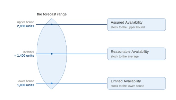
Figure 2. Stocking to the Forecast Range: the three availability strategies and where each sets the buffer.

A worked numerical example below makes the three buffer sizes concrete for a single item across the three strategies.

Consider a single item with an average demand of 100 units per day and a replenishment time of 14 days. The Forecast Range over the replenishment time runs from a lower bound of 1,000 units to an upper bound of 2,000 units, with an average around 1,400 units. The same item, under each of the three item strategies, produces three different buffer sizes, and three different standing investments. The numbers below are illustrative.

StrategyBuffer sizeBuffer coversStanding investment at $5/unit
Assured Availability2,000 unitsUpper bound of Forecast Range$10,000
Reasonable Availability1,400 unitsAverage of Forecast Range (starting point)$7,000
Limited Availability1,000 unitsLower bound of Forecast Range$5,000

The same item under Assured Availability ties up twice the working capital of the same item under Limited Availability. The customer commitments differ accordingly. The annual throughput against buffer cost ratio, developed later in The Nature of Inventory Investment, is what makes the standing investment legible against the return.

Replenishment Is the Shared Mechanism

This point is easy to lose: replenishment and fast response are the operational mechanism for all three strategies. Limited Availability does not mean “no replenishment,” and Reasonable does not mean “loose replenishment.” The key is a fixed buffer per item (or Like Product Group), covering the on-hand stock, the stock in transport, and open orders to the supplier. A sale of eleven units triggers a request or purchase order for eleven. The buffer holds the same size from day to day, unless an explicit decision changes it.

Assured Availability does not mean “tight replenishment of a kind the other two do not get.” Every item the distributor chooses to carry, regardless of strategy, is held against a buffer, depleted by actual consumption, and replenished based on what was consumed. The basic mechanic does not change.

What changes is the parameters: how big the buffer is, how the size is chosen, and what triggers operational action. Those parameters reflect the strategy. The mechanism does not.

The Critical Role of Buffer Management Priority System

The replenishment move itself should run as frequently as possible, from the central warehouse, a local warehouse serving the area, or the supplier, to every store. In most distribution chains this means thousands of different items, replenishing what was sold the day before.

In practice the daily transport often cannot move everything sold yesterday, because capacity of people or vehicles falls short or the source itself lacks inventory. So, a priority system is needed: which items must go today, and which can safely wait for tomorrow’s transport.

Buffer Management, using the buffer status ((Buffer minus On-Hand)/Buffer), paints that priority by color: Green least, Yellow medium, Red highest. Which raises the question: when an Assured Availability item is Red and still cannot be transported today, what then? For such cases an Expediting Policy has to be in place.

Expediting Policy

Expediting, meaning accelerating a replenishment when on-hand stock is at risk, is a real operational tool with real costs: money, management attention, supplier pressure, and the risk of becoming the default rather than the exception. The policy on expediting should follow the strategy, not the buffer color alone.

Assured Availability: the commitment is that the item is available whenever the customer wants it, so a buffer trending toward depletion, a Red status, warrants a check whether expediting is called for. While the item is Red, the replenishment may already be on its way and no action is needed; in other cases a special transport must be initiated to prevent a shortage.

Reasonable Availability: do not expedite as a routine action. The strategy already accepts occasional stockouts; a depleting buffer is information that the buffer may need adjustment, not a trigger for urgency. Since Reasonable Availability covers a large share of most assortments, treating every warning as an alarm would generate continuous urgency at a cost the strategy does not justify. Practically, a Reasonable Availability buffer needs only two colors: Green up to 50% penetration, Yellow above it. No Red!

Limited Availability: do not expedite. The strategy is built on the recognition that surplus inventory poses real financial risk, and expediting would defeat the purpose. Replenishment runs normally, without buffer management. Whether the buffer is good enough is judged by data analysis: the number of days the item was short, and the cost of expired items scrapped.

Buffer Adjustment Over Time

Buffers are not static. Demand patterns change, supply conditions shift, and a buffer that was correctly sized last quarter may be wrong this quarter. The system should adjust, but the adjustment discipline matters as much as the adjustment itself.

The principle: do not make small changes. A 5% or even 15% adjustment to a buffer is below the noise floor of demand variation. It costs operational attention to implement, produces no visible benefit, and trains the system to fiddle. The minimum adjustment threshold should be 20%, large enough that the change reflects a real signal in the demand or supply data, not statistical noise.

One caution governs every adjustment: the sales record doesn’t always reflect the demand record. When an item was short, the system recorded no sale, but the absence of a recorded sale does not mean the absence of demand. Reading raw sales through a period of poor availability creates a dangerous loop: low availability suppresses recorded sales, the lower recorded sales appear to justify a smaller buffer, and the smaller buffer produces more stockouts. Before the data drives any adjustment, it is critical to consider whether shortages prevented demand from being fully satisfied and correct the record for those periods.  

Assured Availability is a commitment made by the distribution company to its customers.  When an Assured Availability item is short, even for just one day, that commitment has been violated!  So, an analysis of what caused the shortage has to be carried out.  The decision on the table is whether to increase the buffer, because of either too high a fluctuation in the demand or a delay in the replenishment, or to wait for more cases, in order to maintain the stability of the system. When the cause sits on the supply side, the diagnosis matters even more, because the failure can be structural: a supplier losing its grip, a central warehouse that has moved to less frequent shipments or a failure of operations. Where the shortage was caused by a delay in replenishment despite a Red buffer status, managerial action is expected, to ensure such a delay is not repeated.

Dr. Goldratt developed the Dynamic Buffer Management (DBM) algorithm, based solely on the daily buffer statuses recorded within the replenishment time. DBM answers when a buffer change is called for; by how much it should change was never resolved, because that answer requires reading what actually changed, the demand or the supply or both, and estimating by how much. This is where AI can improve on the algorithm: recommending not only when to change the buffer, but by how much, and pointing to cases where a tighter management of operations is called for. It is important to remember: the appropriate stock buffer is impacted by the uncertainty in both the demand and the supply. This makes it a worthy target for AI, especially for the buffers of Assured Availability items.

But the AI analysis must also consider the requirement for stability. This means recommending a change only when the data suggests a movement of 20% or more in either direction, not a 7% twitch in the moving average!  This is a lesson that AI has to consider: respond to signal, not to noise. The threshold makes the signal recognizable. We assume both Goldratt and Prof. Deming would agree.

One boundary on the AI’s role needs stating. An algorithm extrapolates from what it has seen, and a novel disruption is precisely what it has not seen: were the Strait of Hormuz to close and block supply for weeks, no history of buffer statuses would tell the system what that event means. Reading a disruption of that kind, and deciding what it demands, remains human judgment. The AI watches the common and expected uncertainty; the exceptional kind still belongs to management.

For Reasonable Availability items, the occurrence of a shortage is normal, on the assumption that all, or most, of the customers find a good-enough substitute in the available assortment. For a distributor whose customers do not substitute, this check does not apply and the item belongs under Assured or Limited.  That key assumption, that a shortage of a Reasonable Availability item does not cost the sale, has to be checked. The check belongs at the level of the assortment, not the individual item: as long as the availability of the assortment is good enough, say more than a third of the members are available, daily sales should be about the same as when the assortment is fully, or nearly fully, available. This can be checked statistically, by comparing the assortment’s sales in periods when its availability was relatively poor against periods when it was relatively good. When a certain level of shortages visibly pulls the assortment’s sales down, the response is to widen the assortment, or to increase the buffers of the members that matter most to customers. The same check can reveal the opposite: the assortment may simply be too big. With, say, only half the members present, sales may even improve, because a smaller choice is easier to choose from.

Here also a key underlying rule should be employed: any change should be significant.  Small and frequent changes are not effective for managing the real-life common and expected uncertainty.

Measuring What Each Item-Strategy Actually Delivers

The system should inquire whether each item-strategy delivers the expected value, so new management decisions can be evaluated and eventually made.  A good performance measurement would be useful.

For Assured Availability items: track the actual stockout rate; the measurement asks whether Assured Availability is in fact happening. A persistent stockout rate above near-zero signals an undersized buffer.

For Reasonable Availability items: track how often the item is actually available. The strategy expects stockouts, but the strategy also has a useful availability target: most of the time. A Reasonable Availability item that is available 75% of the time is performing as the strategy intends. An item that is available 30% of the time is signaling that the buffer is undersized.

For Limited Availability items: track whether surplus is being avoided. The measurement asks whether the standing buffer depletes reliably before it ages, expires, or obsolesces; consistently accumulating surplus signals an oversized buffer. The opposite failure also exists: no scrapped items, but availability below, say, 10%, a buffer too small for the item’s role.

These per-group measurements keep the system honest over time, and they are the data that justifies each strategy assignment to finance, operations, and the executive team, by showing that each strategy is doing what it claims.

Application to Specialized Distributors

The three strategies fit retail-oriented distribution well: grocery, fashion, hardware, where the distributor serves a large anonymous customer base. They also fit specialized distribution, such as parts for older car models, specialty industrial supplies, and contractor materials, but there the operational form can look different, and the difference needs to be named.

Specialized distributors typically know their customers. A customer looking for a specific part for an older car model is rarely substitutable, but often willing to wait if the wait is bounded and predictable: “I can have it for you in two weeks” is acceptable in a way that “we usually have it; sorry, we’re out today” is not. Reasonable Availability fits awkwardly here: the cost of an unexpected stockout to the relationship is high, while the cost of an honest order-on-demand commitment is low.

TOC readers will recognize the manufacturing parallel: Make-to-Availability (MTA), items always kept in stock, and Make-to-Order (MTO), items produced on customer order with a known lead time. The same distinction serves specialized distribution: always-stocked items are the equivalent of MTA, Assured Availability, while items sourced on customer order with an honest lead-time commitment are the equivalent of MTO. Committing to a lead time, of course, requires supply reliable enough to stand behind it.

The strategic logic (commit, partially commit, or do not commit to standing inventory) does not change for specialized distributors. What changes is the operational expression of “do not commit.” In retail, Limited Availability typically means carrying the item selectively; in specialized distribution it often means an explicit order-on-demand arrangement with a clearly communicated lead time. Both are honest, and both honor the same decision: commit something other than standing inventory to this item.

For the Skinny Tail items a specialized distributor cannot economically hold alone, two operational answers preserve availability without a standing buffer at every location. The first is accumulation. Where the network spans a large area with a central warehouse, the Skinny Tail can be stored only at the center and shipped to a store when a customer order arrives, an effective, doable MTO solution. And where several distributors serve the same need (spare parts for older car models is the classic case), they can pool those slow movers at a single shared location, where the combined demand makes affordable Assured Availability none of them could justify alone.

The second is fast response: rather than stock the item, commit to replacing it quickly, a make-to-order arrangement with a short, dependable supplier, often just a few days. For the customer who needs a part for an old model, a reliable three-day delivery is rarely a lost sale. Both answers express the principle running through this paper: availability is managed by holding stock, by accumulating it where demand aggregates, and by responding fast where it does not, with the buffer sized to whatever availability the item’s strategy calls for.

Seasonality and Operational Adjustments Needed

Some items have seasons. Their demand pattern is not the steady distribution that buffer sizing assumes by default but a predictable rise, peak, and fall over a defined window. The underlying logic does not change for these items, but several operational adjustments are necessary to handle them well.

Buffers must be increased before the season begins, because the off-season buffer will be depleted quickly once it starts. Time the increase close to the season, according to the replenishment time. Earlier accumulation ties up cash and warehouse space unnecessarily (necessary in manufacturing, where seasonal capacity is the constraint, but distributors do not need that lead time); later accumulation risks running out at the season’s start, when customer expectations are highest.

Within the season, some commitments may shift when shelf space becomes an active constraint at the peak. The seasonal fast-movers get intensified focus to maintain availability, and several Reasonable Availability items may need an Assured-style operation, because this is precisely when they are sought, while other Reasonable items in the category may receive less commitment than usual while space is tight.

The items that peak are usually a recognizable subset, the seasonal fast-movers, whose demand rises sharply for the window and subsides. They justify the pre-season increase and the in-season attention: they carry the bulk of the season’s throughput, and a stockout at the peak is a stockout at the moment the customer most expects the item. The rest of the seasonal category can stay on its normal strategy; raising those buffers in step would tie up cash and space the season does not repay.

End-of-season demands the opposite adjustment: reduce the raised buffers back to their previous level one replenishment time before the expected end. Shipments arriving at the season’s close become Limited Availability items by default, surplus that should never have been ordered. Ordering steadily through the season’s tail leaves leftovers competing for space and tying up cash all off-season.

Because the peak pressures warehouse space, the season should be planned explicitly, with shelf space for seasonal and non-seasonal items alike. With the increase timed close to the start and the drawdown well before the end, the peak is absorbed without disrupting the rest of the operation.

Transportation and Replenishment Flow

Availability commitments require good control of the physical movement of inventory that sustains them. Earlier chapters covered what to commit to and how to size and adjust the buffers; this chapter covers how the goods actually move and how transportation choices either sustain or undermine the strategic commitments the distributor has made.

Assured Availability depends on the ability to move inventory where it is needed, sometimes urgently. Local buffers thin under demand spikes, and the central warehouse must be able to send emergency shipments when they do. The cost of emergency transportation is part of the cost of the commitment. A distributor who balks at emergency shipment costs and lets local stockouts persist is committing to Assured Availability only conditionally and the customer experience reflects it.

Central-warehouse replenishment and selling-point replenishment are different mechanisms with different rhythms. The center replenishes from suppliers: its demand, aggregated across all selling points, is more predictable but supplier lead times can run to weeks domestically and many months for imports and specialty items. The selling points replenish from the center: local demand is choppier, since one sales event can drain a local buffer, but the center’s replenishment should be short and predictable, sometimes a single day. Buffer sizing differs accordingly: central buffers cover the long supplier time over steadier aggregated demand; selling-point buffers cover the short central time over local more variable demand.

Supplier relationships are inseparable from transportation. How fast will the supplier ship if asked? Will it accept emergency orders? Small quantities quickly, or only full pallets or even truckloads? The answers shape central-warehouse buffer sizing: a supplier who ships a small emergency order in two days permits a smaller central buffer than one who ships on a four-week schedule. The supplier-side question is part of the replenishment design.

The ‘minimum batch,’ so prominent in manufacturing, is also critical to fast replenishment between the central warehouse and the local distribution centers or stores. Any minimum order quantity can delay replenishment and indirectly affect buffer sizing. Sending ten units to cover a two-unit sale may be justified by the right package size, protection in transit or loading efficiency but the resulting problems must be weighed: more trucks, or shipments delayed for lack of them, and DCs or stores forced to hold more than the buffer, pressing on limited space.

Transportation policies, including the minimum transport batches, should be developed, and periodically re-evaluated, with one clear purpose: making the response to any sale at any store fast enough to sustain the required availability.

Transportation frequency is a strategic choice with costs on both sides. More frequent replenishment reduces local buffers but raises transport cost; less frequent does the opposite. The right frequency is not the one that minimizes cost: more frequent replenishment shortens replenishment time, which improves availability from the same or smaller buffers, winning sales that would otherwise be lost. The real comparison is added transportation cost against the throughput better availability produces, plus the cash freed by smaller buffers. Treating transportation purely as a cost to minimize undermines strategic commitments made elsewhere.

Transportation connects directly to the critical resources discussed in the chapter on inventory investment: faster, more frequent transportation frees cash by reducing the buffer each location needs, but transportation is not free either and the right arrangement balances both against the strategic commitments the distributor has made.

Conclusion: Turning Uncertainty into Advantage

The argument of this paper compresses into a few sentences. Demand and supply are uncertain; a forecast is a range rather than a number, and the honest response is a system that replenishes against actual consumption and holds buffers sized to the uncertainty each item carries. Because a stockout is not necessarily a lost sale, not every item deserves the same commitment: three named strategies, Assured, Reasonable, and Limited Availability, make the choice explicit, four sequenced decisions place every item under one of them and a standing financial measure keeps each choice honest about the capital it ties up. The error was never in choosing a less-than-perfect strategy for some items; the error is in not choosing deliberately. Availability is a decision, not a default.

Not all of this is new. Much of what the approach relies on (the Replenishment Solution itself, buffer management, the throughput frame, the treatment of cash and space as critical resources) is established TOC. The contribution is to organize it into a way of managing availability on purpose, and to add the few new pieces where the existing solution ran out. Each closes a specific gap. The three availability strategies give the distributor a way to commit, on purpose, to less than full availability, which the Replenishment Solution, built to protect every stocked item, never offered; this is what lets the solution reach the tail. Two-layer buffering commits availability to a set rather than an item, either a Like Product Group, where one available member is enough, or a whole assortment, where the richness of the choice itself is what must be protected, so that slow items which could never justify a standing buffer alone earn their place inside the set. The assortment managed as a counting buffer, whose units are members rather than units of stock, extends buffer management to variety, a quantity it had never measured. These are the claims the paper stands behind; everything around them is the established solution, used as such.

The cost of not making these choices deliberately is rarely dramatic, which is exactly what makes it dangerous. Two patterns recur.

The account that went quiet. A regional contractor who had been a reliable customer for years gradually reduced their purchases. When a sales rep finally asked, the answer was revealing: “You used to have everything we needed. Now we never know what you’ll be out of. It’s easier to consolidate with a supplier we can count on.” No one had decided to stop serving contractors. Individual item cuts, each defensible on its own, had aggregated into a weaker assortment that no longer met the customer’s needs. The customer did not complain. They simply left. An explicit commitment to a customer segment prevents this, because each item decision can then be weighed against whether it serves the customers the company has chosen to serve.

The slow erosion of identity. A distributor that had built its reputation on depth (“if we don’t have it, it doesn’t exist”) found that reputation fading. No one had decided to become a shallow generalist. But years of tail pruning, each round justified by velocity metrics and margin thresholds, had gradually hollowed out the assortment. Longtime customers noticed; new customers never knew what the company had once been. A market position the company had built over decades eroded through a thousand small decisions, none of which felt consequential at the time. Making the strategic role of each category and item explicit prevents this, so that depth-as-competitive-position is preserved rather than chipped away one velocity report at a time.

Consider the distributor that made the shift. Facing the same eroding tail, it stopped pruning by velocity and instead gave every item an availability strategy: Assured for the few hundred (or thousands when the full offering is > 15,000) items its chosen customers counted on, Reasonable for the broad middle, and Limited, sourced on order rather than stocked, for the long tail it had been abandoning. Total inventory did not climb; it moved, out of overstocked slow movers and into the buffers that protected the relationships that mattered. The contractors who had been consolidating their purchases elsewhere came back, because what they needed was on the shelf again and the space freed from dead tail stock funded deeper coverage where coverage paid. Nothing about the demand had changed. Only the decisions had.

These costs are paid by distribution companies every year, in revenue lost to competitors and in market positions that erode. No approach will make every uncertain decision turn out well; uncertainty guarantees that some will not. What this approach prevents is the silent cumulative loss that comes from managing the tail without one.

None of this comes free, and the approach has requirements and limits. It rests on reliable consumption data; replenishing against what actually sold is only as good as the signal of what sold. It works best where inventory can be aggregated, at a central warehouse or pooled location that lets demand average out before it is committed to a shelf and it asks more of networks that cannot. Above all it takes discipline: an availability commitment means nothing if a slow-item flag is allowed to cut it. A flag can prompt a review; it does not, on its own, change the strategy; only a re-decision does. An item being slow is not in itself a reason to drop it from Assured Availability; that is precisely the reflex an explicit commitment exists to prevent. And it is built for the uncertainty distributors live with every day, the ordinary, recurring variation in demand and supply, not the rare, dramatic shock.

Where to begin is simpler than it sounds. Sort the catalog by how demand behaves, what averages out and what does not, rather than by volume. That sorting sets the starting point, not the strategy: an item whose demand never averages out can still earn Assured Availability when its role justifies the cost. Give each of the three groups its availability strategy. And start where it matters most: the handful of items the customers you have chosen to serve count on you to have. The rest follows from there.

That is what this paper has been about. Distribution has always lived with common and expected uncertainty. The distributors who treat it as something to be named, structured, and managed, rather than forecast away or absorbed by reflex, are the ones who turn the uncertainty everyone faces into an advantage few capture.


What makes manufacturers unhappy about their ERP systems

Switch on captions if you’re watching this video on silent mode.

After you’ve invested hundreds of thousands into your own ERP system, it’s clear you wouldn’t want to find out that there’s a much better alternative on the market. Fortunately, it is not easy for an SME to replace their ERP, and large clients hate it even more. But, the reputation of the ERP company is meaningful for new implementations, and for being able to add more value to their existing clients, by adding applications that either add new required capability, or solve a current problem. 

The simple truth is that most ERP systems are necessary for running businesses, but they fail to yield the full expected value to all clients: to be in good control of the flow that generates the revenues.  

I’m looking forward to your comments here or on my Linkedin post.

Fundamental Default Gap 

When I encounter an ERP system for the first time, I first check whether it helps its user overcome Two Critical Challenges. With rare exceptions, a manufacturer who can’t handle these challenges is inherently fragile, where external factors determine the moment of a break.

All organizations have to make commitments to their clients. Part of such a commitment is the amount of the product or service to be supplied and its overall quality.  Another important part is the time frame for the delivery. There are two broad possibilities for the time frame: either immediately whenever the client asks for it, or a promise for a specific date in the future.

This very generic description defines Two Critical Challenges:

  1. WHAT TO PROMISE: what can we promise our clients, while ensuring a good chance of meeting all commitments?
  2. HOW TO DELIVER WHAT WAS PROMISED: once we have committed to a client, how can we ensure fulfilling the delivery on time and in full? 

It may seem that if you have a good answer to the first challenge, then the delivery is pretty much ensured.  Well, consider Murphy’s law: “Anything that could go wrong will go wrong.”  We are facing a lot of uncertainty, so following the plan is never just a straight walk, you need to deal with many things that go wrong, but that doesn’t mean that you cannot deliver as you’ve committed to. It just means you need to quickly identify problems and have the means to deal with them, still keeping the original commitment intact.

This article focuses on manufacturing companies, even though distribution companies face similar needs. Actually, most service companies also have similar issues with making commitments and then meeting all of them.

The potential value of any ERP package for manufacturing is to provide the necessary information, based on the actual data, to lead Operations to do what is required for delivering all sales-orders on time and in full, without generating too high cost. In other words: ERP should support the smooth and fast flow of goods, preferably throughout the whole supply chain, and at the very least, manage the flow from the immediate vendors to the immediate clients.  

When properly modelled and used, the current ERP systems provide the production planners with easy access to all the data about every open manufacturing order and the level of stock of every SKU. The data also covers the processing and setup times for every work center, again when being properly input by the user. So, capacity calculations can be performed with current technology.

Question for ERP brands and developers: 

How does that huge amount of data, currently collected by your ERP, help to overcome the Two Critical Challenges for your customers?

If this question sounds too rhetoric, I encourage manufacturers to share their experience on how they adapted to work around the gap after it was by default inherited with a chosen ERP package.  

Manufacturing organizations seem to be very complex. While outlining the whole process from confirming a sale-order until delivery isn’t trivial, the ERP tools are good enough to handle that level of complexity. But synchronizing all the released manufacturing orders, which compete for capacity of resources, is a major problem. Consequently, even though timely delivery of one particular high priority order is not a problem, achieving an excellent score on OTIF (on-time, in full) seems very complicated.

So, in order to be able to answer the two challenges there is a need to have good control on the capacity of resources.

Promise, then deliver

Measuring capacity is not trivial.  Just having to deal with setups adds considerable complexity.  During the 90s, along with powerful computers with great ability to crunch millions of data items, the idea of creating an optimized schedule, taking into account all the open sales-orders, going through each order routing, considering the available capacity at the right time, came to life with a new wave of software called APS (advanced planning and scheduling systems). These systems were supposed to yield the perfect planning, meaning it could be performed in a straightforward way, accomplishing all the objectives of the plan. If this could really work, then the second challenge would have been solved as well.

However, the APS systems eventually failed. Some claim they could still be used for inquiring about what-if scenarios.  Problem is: it can tell you what definitely wouldn’t work, for instance because of lack of capacity of just one resource. But APS failed to predict the safe achievement of all commitments, so its main value was, at most, quite limited.

The reason for the failure of all the APS is that on top of complexity of managing the capacity of many resources, there is considerable uncertainty, and any occurrence of a problem would mess up the optimal plan.

Relative to the APS programs, the development of ERP aimed at integrating many applications using the same database, without considering the capacity limitations and without striving for the ultimate optimal solution. Some ERP programs have widened the ability to model more and more complexity, others are still going with the basic structure.

Even when we have excellent data, and effective ERP tools, managing the uncertainty is quite a tough task. It is always tough – no matter the plant type or industry – because of the complexity of monitoring the progress of so many manufacturing orders. Every production manager struggles with the ongoing need to decide what work order has to be processed right now.  This also means that processing other work orders is delayed.  When the market demand fluctuates, when problems with the supply of materials occur, or when machine operators are absent, the production manager must have a very clear set of priorities, and certain flexibility with time, stock, and capacity to be able to respond immediately to any new problem. The objective is still valid: delivering everything according to the commitments to the client. 

Note, if we come up with a solution to the second challenge (2. How to deliver what was promised), then we might also understand better what truly limits our offering (and commitment) to the market. Once we know that, we can come up with an effective planning scheme where every single promise made by our sales people is pretty safe.

This is where the insights of the Theory of Constraints (TOC) come to our rescue.

Key insight #1:
Only very few resources, usually just one, truly limit the output of the system.  

The recognition of the above statement effectively simplifies monitoring the flow. In TOC we call that resource the ‘constraint.’ Certainly, the capacity of the constraint should be closely monitored. Several other resources should also be monitored, just to be sure that a sudden change in the product mix won’t move the ‘weakest link’ to another resource. The vast majority of the other resources have much less impact on the flow, as they have some excess capacity, which can be effectively used to fix situations when Murphy causes a local disruption. 

One additional understanding from that key insight: the limited capacity of the constraint is what could effectively be used to predict the safe-time where the company can commit to deliver. More on it will be explained later.

Key insight #2:
An effective plan has to include buffers to protect the most important objectives of the plan.

Buffers could be time, stock, excess capacity, excess capabilities, or money.

In manufacturing we can distinguish between make-to-order (MTO) and make-to-stock (MTS).  The vast majority of the manufacturing organizations produce both for order and for stock, sometimes within the same work-order there are quantities promised to be delivered at certain dates (MTO), while the production batch also includes items to cover future demand (MTS). This creates quite a lot of confusion, and makes the life of the production manager, who is required to locate all the parts that belong to a specific sales order, a never-ending nightmare. 

You will be surprised but even the most popular ERP systems do not differentiate between MTO and MTS. If you wonder why obviously an MTS company manages its production the MTO way, check their ERP system default (and watch a follow-up video below for more explanation on this).

My team discovered one ERP system, Odoo, that distinctly differentiates between MTO and MTS. This distinction makes Odoo a strong contender for a platform on which to build the necessary features that address the key insights. I’m excited to see how effectively these features are already responding to two critical questions, and I look forward to discovering what more we can achieve in the future. Generally speaking, this capability is also possible with other ERP systems as well.

Every MTO order has a date that is a commitment. Considering the uncertainty there is a need to give Production enough time to overcome the various uncertain incidents along the way, including facing temporary peaks of load on non-constraints, quality problems, delays in the supply and many more. This means necessarily starting production enough time before the due date to be confident that the order will be completed on time. That time given to Production with a good confidence is called Time-Buffer, and in manufacturing it includes the net-processing time, because in the vast majority of manufacturing environments, the ratio of net-processing time to the actual Production Time is less than 10%. Thus, the order release date should be: due-date minus the time-buffer-days.  We highly recommend not releasing MTO orders before that time, otherwise significant temporary peaks on non-constraints will be created.

Make-to-stock requires maintaining a stock buffer. The definition of the stock buffer includes on-hand plus open manufacturing orders for that item. Thus, when a sale automatically triggers the creation of a manufacturing order for the same SKU, then the stock buffer is kept intact.

Key insight #3:
The status of the buffers provides ONE clear priority scheme!

In TOC we call it Buffer Management. The idea is to define the status of the buffer as the percentage of how much of it is left. As already mentioned, in manufacturing the net processing time (touch time) of an order is a very small fraction of the actual production lead time. The most production time is spent waiting for the work-centers to finish previous orders. Thus, if a specific order becomes top priority, the wait time for that order would be significantly cut and so would the lead time.  

MTO orders use time buffers, while as explained earlier, MTS orders use stock buffers. Ideally, we should monitor both MTO and MTS orders in the same queue as you see in the Picture 1 below. When only one-third of the time-buffer or less is left until the delivery date, or the on-hand stock is only one-third or less of the stock buffer, the buffer status of that order is considered RED, meaning it has top priority.  Once that red order gets the top priority the wait time is dramatically cut. The production manager facing a list of several red orders could decide to take expediting actions to ensure a fast flow of the red orders, so all of them will be completed by the due date.

For MTS orders the buffer status is the percentage of the on-hand stock relative to the stock-buffer, which also includes the WIP (work-in-process). Following the one priority scheme, using both stock and time buffers significantly improves the probability of excellent delivery performance. This happens mainly when some level of excess capacity exists, even on the constraint, and more so on the few other relatively highly loaded resources. However, when the demand goes up, then at some point in time the number of orders in RED increases sharply.  When this situation happens, it radiates a clear warning: There is no way to meet the commitments as long as there is no significant increase in capacity.  We can call this kind of warning “too much Red.”

List of manufacturing orders prioritized by Buffer consumption (screenshot from TOC app in Odoo)
In Buffer Management, penetration of the red-line initiates expediting of a particular manufacturing order (and related work orders). When the number of RED orders – those that have crossed the red-line – goes up sharply, a true bottleneck is emerging. (Picture 1)

Key Insight #4:
Monitoring the size and trend of the Planned-Load of the constraint, and few other highly loaded resources.

The Planned-Load of a specific critical resource is the total hours required to process all the confirmed sales-orders. This is done simply by going through all the backlog of orders and adding the required hours of work of that resource to process the orders.  The most critical resource, the constraint, is expected to have the highest number of hours required for processing all the existing orders. The Planned-Load could be expressed as the date where we expect the critical resource to finish processing all the confirmed demand.

Note two critical advantages from the Planned-Load that benefit and align Production and Sales:

  1. We get an accurate prediction of the lead-time for a new order!  

When a new order appears in the backlog, then in most cases it will be processed by the critical resource only after all the existing demand (confirmed orders) have been processed. When we add to the Planned-Load some extra time (usually half of the time buffer for that order), covering for the processing time of the constraint and going through all the rest of the routing, we get a safe-date we can commit to.

  1. Watching the trend of the Planned-Load provides us with signals on the overall trend of the market.  

The Planned-Load should be re-calculated every day. The difference between today’s planned load and tomorrow’s is that the orders processed by the resource today disappear from the calculation, while new orders arriving today are added to it. When the Planned-Load of the constraint increases (see the right screen in Picture 2), it means more orders are coming than what the constraint has been able to process. If such a trend is consistent for some time, it might mean: a bottleneck is emerging. You either won’t be able to deliver on time (and suffer customer dissatisfaction), or you will be forced to increase the lead time (and consequently lose some business when your competition remains faster). When the trend goes down (as shown in the left screen in Picture 2), it means less orders are received from the market, and then it is possible to deliver faster.

Planned Load graph of the Capacity Constrained Resource generated by TOC app in Odoo.
The trend of the Planned Load of the Capacity Constrained Resource (CCR) is an immediate indication whether the CCR will become a bottleneck or whether sufficient protective capacity still remains (Picture 2).

Depending on the trend, the company should trigger a proper managerial initiative:

  • either to increase the capacity of the constraint, possibly also the capacity of one or more of the other critical resources, as we don’t want them to become bottlenecks,
  • or find ways to attract more orders and more new customers. Note, less loaded constraint means a shorter lead time. In markets where supplier response time and reliability matter a lot, a shorter lead time magnetizes new orders. This means if Sales and Operations activities are synchronized, any drop in demand could be just temporal. 

Balancing carefully between demand and capacity

The combination of monitoring both the number of red orders and the Planned-Load yields a powerful piece of information on the stability of the organization, regarding the sensitive balance between demand and capacity.  The advantage of Buffer Management is that it doesn’t depend on the quality of the vast majority of the ERP data, only on the consumption of time or stock. The advantage of the Planned-Load is its ability to issue a warning earlier than Buffer Management, giving the managers more time to react, including the option to add temporary capacity.

The actual value from the combination of Buffer Management and Planned-Load has been thoroughly checked using the MICSS simulator, developed by me during the 90s for testing various production policies and their impact on the business.  When the market demand starts to grow, after some time the number of red orders suddenly increases. At that time the current delivery performance is still adequate. But after running the simulation for one or two more weeks, the disaster in the delivery is clearly seen. I hope and wish your factory’s reality is much better than that!

The four key insights could be effectively used to vastly improve the value and skyrocket ROI of any modern ERP system, still using most of the capabilities and algorithms of the original ERP.  

My team and I at Enterprise Space, Inc. are determined to continue adding new algorithms and data visualisations to an ERP system that would focus the managers to the truly critical issues.

The next phase of value to the customers would be detailed by a subsequent article on how to support decisions when additional new sales initiatives are evaluated, predicting the net impact of those decisions on the bottom-line, taking revenues, cost and capacity into account, considering also the level of uncertainty.

Switch on captions if you’re watching this video on silent mode.

Fighting Uncertainty as a Critical Part in Managing Organizations

By Eli Schragenheim and Albert Ponsteen

The article is based on the webinar “Fighting Uncertainty in Organizations, Including Matrix Ones, to Achieve Excellent Reliability.”

This article explores managing uncertainty in organizations. Although the key ideas are generic, special emphasis is on multi-project environments. Drawing from Dr. Goldratt’s philosophy, it emphasizes knowing something but never everything. The authors spotlight overlooked “common and expected” uncertainties like equipment malfunctions and seasonal variations. These seemingly minor uncertainties can cumulatively impact performance and disrupt detailed planning. The “Domino Effect” describes how these uncertainties can combine and amplify challenges. The article advocates for adaptive strategies and the use of buffers as protective measures against unpredictable organizational challenges.

1. The Philosophy of Knowing and Not Knowing

Never Say ‘I Know’ and Never Say ‘I Don’t Know’: You always know something but never everything.

The principle of never saying “I know” or “I don’t know” comes from a nuanced understanding of the constant uncertainty we live in. The founder of TOC, Dr. Goldratt, emphasized the point of “never say I know” as a reminder to stay humble about our knowledge. However, he was equally insistent that we usually know something about the subject matter. This balance between acknowledging our limitations and recognizing our abilities is essential in navigating uncertainty. It helps us begin somewhere rather than getting paralyzed by what we don’t know.

“When Dr. Goldratt came to me and asked, ‘Eli, how long will it take you to develop a new feature’, I hesitated. I was well aware that part of my code was complex and any addition would be risky. My first inclination was not to give him a number. But Goldratt insisted, ‘At least you can tell me whether it’s closer to two hours or two years.’ That’s when it clicked for me. He didn’t need a precise number; he needed a sense of the time frame. So, I told him, ‘It will not be more than two weeks.’ And he replied, ‘OK, this is what I wanted to know’.” Eli Schragenheim

This paradigm shifts our perspective on how to approach uncertainty. It equips us with the mindset to acknowledge that while complete knowledge is unattainable, we must not let our gaps in knowledge deter us from making decisions or taking actions. It is this very mindset that shapes our approach to tackling uncertainty in organizations.

Read more at:

https://elischragenheim.com/2016/01/09/never-say-i-know-and-the-limitations-of-our-reasonable-knowledge/

2. Identifying the Huge Impact of Common and Expected Uncertainty

In the preceding section, we laid the groundwork for understanding the nature of common and expected uncertainty. Because these uncertainties are considered “part of the job,” there is a tendency to underestimate their impact. The mistake here is viewing them as isolated incidents rather than cumulative forces that can weigh heavily on the organization’s performance and planning. Here, we will dive deeper into understanding its mammoth impact on organizational planning and performance. Although the emphasis is on multi-project environments, the key ideas are generic.

The Incidents That Don’t Surprise Us

Often, these are the uncertainties that are most overlooked precisely because they are so familiar. These could range from employee turnover, equipment malfunctions, or even seasonal variations in sales for businesses. 

“I was approached by a company to investigate why a very important project that should have taken one year actually took five years. Management clearly did not think this was ‘common and expected’ uncertainty; they would have tolerated it for maybe two years. But the professionals who executed the project considered it a huge success. They said, ‘In the U.S., they have been working on it already for more than 10 years, and they are not close to what we have achieved.’ This was enough for me to deduce the team had set a one-year plan, knowing it is excessively optimistic because they were concerned that if they had told it could take five, or even ten years, the project would never have started.” Eli Schragenheim

The lesson is: when you ask for a clear one-number estimation, without defining the level of common and expected uncertainty, then you either might face big surprises or face frequent occurrences, where the project/mission finished exactly on time. The latter case actually means that the mission could have easily finished before the planned time. Both cases cause severe damage to the performance of the organization.

The Impracticability of Detailed Planning

Common and expected uncertainty often messes up the execution of a detailed plan, making the original plan to be almost useless after a relatively short time. The more complex the plan, the more vulnerable it is to disruption from these routine uncertainties. Adaptive planning becomes crucial here. While having a plan is essential, the ability to adapt and modify it in real time is invaluable. The problem is that the intended outcomes and commitments to the market might be negatively affected, harming the reputation of the organization. This section discusses the challenges of planning in an environment filled with common uncertainties and suggests more dynamic, adaptable approaches, which most of the time contribute to achieving the desired objectives.

For instance, suppose the output of the project requires five different inputs from five different teams. What is the probability that the project will finish on time? Any delay in any input would delay the whole project, no matter how early the other teams submitted their inputs. So, what date should you offer reliably? 

The Domino Effect

One of the most underestimated aspects of common and expected uncertainty is how it can accumulate. An employee’s unexpected sick day may not seem that impactful alone. But combine that with a minor delay in raw material delivery and throw in a sudden but not surprising market fluctuation, and you have a perfect storm. This is the Domino Effect in action: individual uncertainties, seemingly manageable on their own, can combine to produce an outcome far worse than any of them could individually. The cascading impact can be particularly detrimental to delivery performance, disrupting schedules and damaging reputation.

The above example of the five teams (see the end of the previous section) demonstrates a typical situation where lateness of one task is not compensated by other tasks that are early. This is the “integration effect.” Another situation for possible domino effect is when the output of a task, while on-time, fails to deliver the planned quantity, thus the subsequent operation has only limited inputs to work on, creating a negative effect throughout the chain. 

Parkinson’s law states that work expands to fill the time allotted for its completion. Practically it means that when a planned task is delayed due to uncertainty, the delay is not compensated by other tasks finishing early. This behavior of Parkinson’s law causes much of the Domino Effect in projects, on top of the two above situations that generates an accumulation of delays.

3. Including Protection Mechanisms, Like Buffers, Against Uncertainty

In the previous section, we highlighted the underappreciated role of common and expected uncertainties in project management. This chapter digs deeper into a powerful tool for mitigating their impact: buffers. Beyond just time, buffers can cover finances, manpower, and more.

Everyday Strategies to Counter Uncertainty

Just as project managers use buffers to navigate uncertainties, we employ similar tactics in our daily lives. These aren’t complex plans but simple, intuitive steps that serve as safety nets for the unexpected.

  • Catching a Flight (Time Buffer). When you need to catch a flight, you usually aim to reach the airport well before the departure time. This accounts for potential traffic delays, long security lines, or other unforeseen events.
  • Preparing Dinner (Resource & Quantity Buffer). When hosting a dinner, you might buy extra ingredients. This accounts for the possibility of some ingredients getting spoiled, the recipe requiring more than expected, or perhaps an unexpected guest arriving.
  • Saving Money (Financial Buffer). Financial advisors often recommend keeping an emergency fund to cover sudden, unforeseen expenses like a broken appliance or medical emergency. This is different from saving money for investment purposes, which is about growing your financial resources over time. The emergency fund acts as an immediate financial buffer, providing peace of mind and stability in case of unexpected setbacks.
  • Carrying an Umbrella (Risk Buffer). Even if the forecast suggests only a 10% chance of rain, you might carry an umbrella when heading out for the day, just in case.
  • Keeping a Spare Tire (Risk & Resource Buffer). Most vehicles come with a spare tire. Even if you never expect a flat, it’s there as a buffer against that potential problem.
  • Having Insurance (Risk Buffer). Be it health, car, or home insurance; the idea is to have a buffer against unexpected damage or health issues.
  • Dressing in Layers (Flexibility Buffer). If you’re uncertain about the weather, you might dress in layers. This way, you can adapt to a warmer or colder environment by adding or removing clothing.
  • Backup Power/Charger (Resource Buffer). Carrying a power bank when out for long hours ensures that even if your phone’s battery depletes faster than expected or if you use it more than usual, you won’t be left without a functioning device.
  • Learning Additional Skills (Skill Buffer). People often upskill or learn things outside of their primary profession. This not only helps in personal growth but also acts as a buffer in changing job markets or if one decides on a career shift.

In short, these everyday buffers help us manage uncertainties and offer peace of mind, reinforcing that while we can’t foresee all events, we can prepare for many incidents.

Buffers Mean Planning Spare of What We Might Need

Buffers are vital tools in project management, used to mitigate various uncertainties. While time buffers are most common, there are several types to know, each targeting specific risks.

Buffer Types at a Glance

Buffers are surplus resources allocated to navigate inevitable uncertainties. For example, a project estimated at 100 work hours might include a 20-hour time buffer for contingencies like absences or technical issues.

“I remember being invited by the Olympic Committee of a country to consult on their planning for the Games. The date was fixed, the world would be watching, but what buffers did they have? You’ll be surprised: Their main buffer was a huge amount of money. Most of which could have been saved with better planning. Sometimes you need to ‘waste’ to create a buffer, but the trick is to waste wisely so as not to incur unnecessary costs.” Eli Schragenheim

By strategically applying buffers—be it a financial buffer for a grand event like the Olympics or a time buffer for a smaller-scale project—managers can significantly enhance the project’s success rates and readiness for unforeseen issues. This real-world example underscores the importance of not only having buffers but also optimizing them to save resources.

The Stigma Against Buffers

Buffers are essential for managing uncertainties, yet they often meet resistance, especially in management circles. This skepticism arises from the belief that buffers are wasteful or overly cautious. When buffers are made visible, trust is crucial; without it, their presence can reinforce negative stereotypes, painting them as budget inflators rather than strategic tools. The key challenge is to reframe buffers as vital elements of proactive planning, dissolving resistance, and promoting a resilient approach to managing inevitable project uncertainties.

The Key New Insight: Include Visible Buffers in the Planning!

Making buffers visible in project plans fosters transparency and effectiveness. Unlike traditional hidden buffers, visible ones enhance project tracking and offer a measurable cushion for unexpected challenges. They also set realistic expectations by highlighting flexibility in planning. This visibility counters the stigma against buffers, framing them as strategic, rather than wasteful. In short, visible buffers improve accountability and project success.

Buffers Are Sometimes Partially Consumed

An important subset of these visible buffers is the partially consumed buffer. These buffers are dynamic and adaptable, offering the flexibility to make real-time adjustments. For example, if a project task initially includes a 20-hour time buffer and only 10 hours are needed, the budget for the 10 hours can be reallocated or saved for future needs. Such flexibility not only allows for real-time optimization but also leads to more efficient resource management. The effective planning and use of these dynamic buffers are key for project success.

Planning visible buffers has to include the issue of where the buffers should be inserted. Protecting every single task within a project is useless. What we really need is to protect the completion of the project. Thinking about what could easily disrupt the safe completion and also ensure the quality of the outcome would lead us to note where the buffers are truly needed. TOC has fully developed methodologies for determining the right location of buffers in projects as well as in manufacturing.

Conclusion

Buffers serve as a crucial mechanism in the armor of project management against the unpredictability and uncertainties inherent in any project. While they are often misunderstood or misapplied, a nuanced and strategic approach to buffering can save both time and resources in the long run. Making buffers visible and understanding that they can be partially consumed allows for a more flexible, robust, and resilient project management approach.

4. Setting Priorities in the Execution Phase, Based on the Actual Consumption of the Buffers

In this chapter, we’ll delve into the critical role of prioritization and buffer management during a project’s execution phase. We’ll emphasize the limitations of relying solely on time buffers and advocate for a real-time dual-buffer approach that monitors both time and capacity.

The Essential Role of a Unified Priority System

Navigating the complexities of multiple projects demands a unified priority system. This system serves as a single source of truth for decision-making and is informed by real-time buffer consumption, guiding efficient resource allocation.

In a multi-project landscape, a unified priority system is indispensable. It provides a stabilizing framework and helps avoid the pitfalls of striving for an elusive “optimal” solution, focusing instead on what’s practically achievable.

Read more:

https://elischragenheim.com/2016/12/26/the-toc-contribution-to-healthcare/

Read more: 

https://www.researchgate.net/publication/228472949_Utilising_buffer_management_to_manage_patient_flow

Monitoring the State of Many Buffers Leads to Identifying Situations Where the Whole Protection Scheme Might Crash.

The effectiveness of buffers relies not just on their existence, but on ongoing monitoring and adjustment. As projects evolve, so should the buffers that safeguard them, meaning part of them is consumed by the incidental delays that have occurred so far. However, when implementing a buffer management system, a single focus on individual projects or processes can be short-sighted. A broader, more comprehensive outlook is necessary for effective risk mitigation and preventing potential cascading failures across the entire protective scheme. We need an early warning that the system might crash.

Monitoring the Buffers

In the context of managing uncertainties in multi-project environments, buffer monitoring is intricately linked with the “fever chart” of Critical Chain Project Management (CCPM). The fever chart graphically represents the consumption of project buffers against the completion of project tasks. By regularly monitoring the consumption of these buffers – whether they pertain to time, resources, or finances – organizations can derive real-time insights into the health and progress of their projects. This visual tool, when intersected with the buffer consumption rate, offers a clear picture of project performance. If the chart indicates a buffer being consumed too rapidly relative to task completion, it serves as a warning signal, indicating potential issues and enabling managers to proactively adjust strategies or allocate resources, thereby ensuring optimal project outcomes.

A modern version of a Fever Chart using infographics by Epicflow

The Hidden Risk: Relying Solely on Time Buffers

Time buffers, often represented through color-coded statuses, may be misleading indicators in a multi-project environment. While they effectively signal potential issues in individual projects, they fall short of capturing systemic risks. A few projects shifting from “green” to “red” may seem like isolated issues. However, when multiple projects turn “red,” it can expose the fragility of the entire system and trigger a cascade of failures. By this point, corrective action is usually too late to avoid widespread disruption.

The Missing Link: Capacity Buffers

Capacity issues, when overlooked, lead to significant obstacles in project management. If these issues are not addressed promptly, they result in what is called a “bottleneck” – a point of congestion where tasks accumulate, leading to delays. For instance, if a particular engineering team is stretched thin, all projects dependent on that team will experience delays. Since capacity isn’t project-specific but shared, a deficit impacts multiple projects. 

Monitoring the level of access capacity provides the missing layer of protection. They alert management to shared critical resources that can derail multiple projects simultaneously. Neglecting to monitor capacity can leave the system vulnerable to unanticipated crashes, making the dual-buffer approach imperative for holistic project management.

Read more: https://www.epicflow.com/blog/once-in-red-always-in-red/

Read more: https://elischragenheim.com/2016/09/03/the-critical-information-behind-the-planned-load/

The Dual Buffer Strategy: A Comprehensive Approach

The most effective buffer management strategy incorporates both time and capacity buffers. This dual approach provides a nuanced, multi-dimensional view of project health, enabling proactive measures to avoid both individual project delays and systemic failures.

Dual buffer representation in Epicflow

Understanding History to Plan for the Future

Understanding the dynamics of capacity buffers to plan the future is incomplete without considering the historical performance of your teams. This data is not just a reflection but a predictive tool, embedding lessons from the past to enrich future planning strategies.

Consider an engineer scheduled for four 8-hour tasks in a 40-hour week. If only three tasks are consistently completed, a gap between planned and actual output becomes apparent. This recurring pattern isn’t a one-time anomaly but indicates a need for reassessment and adaptation in task estimations or effective capacity planning.

The incorporation of historical data ensures that future strategies are well-rounded, combining past performance trends and adaptive responses to uncertainties. This data serves not just as a record but a predictive tool, embedding past lessons to enhance future adaptability and resilience.

In cases where only three out of four planned tasks are consistently completed, it signifies an essential gap between planned capacity and actual output. Such insights lead to a reassessment of the benchmarks set for capacity. Informed by historical performance, adjustments can be made to align with actual output trends. This data-driven approach builds robustness and adaptability, ensuring that project plans are efficient and effective. It prepares teams for unforeseen challenges, enhancing the organization’s agility and responsiveness to change.

Historical performance measured in Epicflow

Conclusion

While time buffers are valuable tools, their utility is severely compromised if capacity buffers are ignored. A dual-buffer system that includes real-time monitoring of both time and capacity is essential for navigating the complexities of multi-project environments. This approach offers a comprehensive safety net, enhancing both individual project success and overall organizational resilience.

5. A More Generic Insight: We Should Estimate the Size of the Common and Expected Uncertainty as a Reasonable Range

The concept of “reasonableness” is subjective and varies from one situation to another. However, when it comes to forecasting, being “reasonable” requires us to rely on judgment informed by both data and experience. Too often, we see forecasts presented as a single number, creating an illusion of certainty that’s misleading. In truth, the term “reasonable” isn’t about aiming for pinpoint accuracy, but about grounding our expectations in reality.

Do Not Overprotect from Very Rare Incidents

Planning against highly improbable events, like your supplier being hit by a tsunami, may not be reasonable in most scenarios. Overpreparing for such outliers can tie up resources and lead to inefficiencies. The key is to prepare for what is most likely to happen. For example, if a supplier promises delivery in two months, a reasonable buffer might be planning for a three-month wait instead. This allows you to prepare for the “expected uncertainty” without spreading your resources too thin.

Use Risk Management Tools to Evaluate High Risks with Very Low Probability

For those black swan events that are highly improbable but catastrophic, other mechanisms like insurance or government protection schemes are more appropriate. These are separate from the day-to-day operational buffers and help shield against large-scale disruptions.

A major realization is: Don’t forecast ONE number -> always use a range!

Forecasts should always be expressed as a range rather than a single point. A range not only provides a more realistic picture but also allows for better planning and resource allocation.

Putting it All Together: The Need for a “Reasonable Range”

When it comes to decision-making, whether it’s forecasting sales for the next month or planning a project, we need to adopt the practice of using “reasonable ranges.” A range provides us with a cushion, offering protection without leading to resource wastage. This is critical, not just in supply chain decisions but in marketing, operations, and human resource management.

Budgets Should Reflect Realistic Buffers

In many organizations, budgets often have a narrow buffer, usually entitled as “reserve,” sometimes as little as 5%. This is usually insufficient for dealing with unexpected changes or opportunities. Budgets need to be more dynamic, with larger reserves that can be deployed when genuinely needed.

Forecasts as Targets: A Double-Edged Sword

Many organizations use forecasts as targets, which can lead to unintended consequences. For example, if you set a two-week target for a project, you can be almost certain it won’t be completed in less time, which is the essence of Parkinson’s law. People will often “use up” the allotted time, sometimes focusing on unnecessary details. Targets should be flexible, allowing for both over-performance and the unexpected.

Measurement Systems Need to Reflect Realistic Expectations

Just like university grading systems, where a score of 84% doesn’t really mean that the student did better than another student who got only 80%, and worse than one who scored 88%, we need measurement systems in the workplace that reflect broader categories. Instead of obsessing over small numerical differences, focus on what is “good enough”, what is “excellent”, and what is “unacceptable”.

Read more: https://elischragenheim.com/2016/04/10/between-reasonable-doubt-and-reasonable-range/

Read more: https://elischragenheim.com/2016/03/09/why-should-the-red-zone-be-13-of-the-buffer/

In Summary

When it comes to forecasting and planning, it’s essential to always think in terms of ranges rather than specific points. This provides a more flexible and realistic framework for decision-making and resource allocation. “Reasonable” doesn’t mean overly cautious; it means well-considered and flexible. As we become more experienced, our sense of what constitutes a “reasonable range” will become more accurate, allowing for more efficient and effective operations across all aspects of business.

References:

[1] “Never Say I Know” and the Limitations of our (Reasonable) Knowledge, Eli Schragenheim (2016).

[2] The TOC contribution to Healthcare, Eli Schragenheim (2016).

What are the fundamental concepts of the Theory of Constraints?

By Eli Schragenheim and Dave Updegrove

Eli.S note: this article is the result of a collaboration between Dave Updegrove and I, on the topic of defining the essence of the Theory of Constraints (TOC). 

We claim that every beneficial insight removes a current limitation that prevents us from achieving value.  The limitations TOC deals with are usually caused by flawed paradigms, or assumptions. 

With this basic insight, Dave and I have looked into the TOC body-of-knowledge, and tried to understand, for every insight, concept or tool, what was the limitation that the particular insight had removed, meaning what value couldn’t have been generated and now, using the new insight, we are able to.

Next step is to understand the flawed paradigm behind the limitation, so we’ll be able to clearly understand the scope of new potential value that can be reached.

We have chosen what we believe to be the most generic concepts of TOC and the limitations, followed by the identified flawed assumptions, behind these concepts, and also the somewhat lower-level insights/concepts/tools they impact.

Three key concepts that address the three fears of every manager: complexity, uncertainty, and conflicts.

Concept 1: Inherent Simplicity.

All systems (for instance, organizations) are inherently simple, despite their apparent complexity.

In systems, a few or even one point (Constraint[s]) controls the performance of the whole system, and a few or even one root cause (Core Conflict[s]) generates the vast majority of problems.

Limitation addressed:

Being unable to predict, in a good enough way, the consequences of an action or imposed change.  This failing to predict consequences vastly reduces the quality of decisions.

Flawed assumption:

Treating our current reality as complex, thus failing to make the efforts to identify the few variables that significantly impact the consequences of any action or change.

We can find and manage the few points controlling the system

Example of following the flawed assumption:

Dividing a complex system into subsystems, assuming, 1) that they are much less complex, and 2) that this can help to predict the local impact of any change; further hoping that optimizing local systems will result in good enough prediction of the impact on the whole.

This expectation is most damaging.

Resulting/affected applications:

The Five Focusing Steps, the Four Concepts of Flow, the Three Questions

Concept 2: Inherent Consistency (Harmony):  

There are no conflicts (or inconsistencies) in reality.

All conflicts (on inconsistencies) exist only in our minds. One or more invalid assumptionsare behind every perceived conflict (or inconsistency).

Limitation addressed:

Having to compromise between two conflicting actions, where each action is necessary to satisfy a necessary condition for achieving a desired common objective.

By compromising we get significantly less value for the desired objective.

Flawed assumption:

We know and accept our perception of “reality.”  Actually, every perception of reality is based on many (hidden) assumptions.  It is possible that challenging just one assumption, meaning creating a situation where that assumption is not valid, opens the way to get much more of the common objective.

The perception of a “conflict” should trigger us to reveal our assumptions and then look actively for a valid (realistic) way to challenge them.

Example of following the flawed assumption:

The seesaw conflict of holding less inventory to lower investment and carrying costs, versus holding more inventory to ensure availability to the system, allowing generating more value.

Resulting/affected applications:

The Evaporating Cloud (Conflict resolution diagram), The Change Matrix / Procon cloud

Concept 3: Inherent Consistency (Harmony):  There are no conflicts (or inconsistencies) in reality.

All conflicts (on inconsistencies) exist only in our minds. One or more invalid assumptions produce any perceived conflict (or inconsistency).

Limitation addressed:

Having to compromise between two conflicting actions, where each action is necessary to satisfy a necessary condition for achieving a desired common objective.

By compromising we get significantly less value for the desired objective

Flawed assumption:

We know and accept our perception of “reality.”  Actually, every perception of reality is based on many (hidden) assumptions.  It is possible that challenging just one assumption, meaning creating a situation where that assumption is not valid, opens the way to get much more of the common objective.

The perception of a “conflict” should trigger us to reveal our assumptions and then look actively for a valid (realistic) way to challenge them.

Example of following the flawed assumption:

The seesaw conflict of holding less inventory to lower investment and carrying costs, versus holding more inventory to ensure availability to the system, allowing generating more value.

Resulting/affected applications:

The Evaporating Cloud (Conflict resolution diagram), The Change Matrix / Procon cloud.

Two Key Tools

Concept 4: Inherent Causality:

Systems are subject to cause-and-effect dynamics.

To understand and manage a system, apply rigorous cause-and-effect logic, governed by the Categories of Legitimate Reservation

Limitation addressed:

Being unable, even when accepting the inherent simplicity, to answer the three questions:

  • What to Change?
  • What to change to?
  • How to cause the change?

Flawed assumption:

Using logic is too cumbersome, subjective, and difficult to quantity, to make it effective in finding answers.

A few simple, learnable logical tools can greatly enhance analysis and provide answers to important questions.

Example of following the flawed assumption:

Attempting to independently solve any undesirable effects (symptoms) in the organization without considering root cause(s).

Resulting/affected applications:

The TOC Thinking Processes, The Three Questions

Concept 5:  Inherent Valuation

By dividing expenses into truly-variable costs and the cost of capacity, an entire system and each of its parts may be properly valued. The focus is on Throughput: the pace of generating goal-units. For commerial organizations throughput is: the periodical revenues minus the truly variable expenses.

Limitation addressed: 

It is very complicated to predict the financial outcomes of a suggested action, trying to evaluate directly its impact on revenues and expenses.  Without a well-accepted procedure to make such decisions, managers would be afraid to use such a complicated analysis. 

Flawed assumption:

Not distinguishing between linear behavior and non-linear.

Subtracting truly variable expenses from revenues (resulting in Throughput), and considering non-truly variable expenses to be part of Operating Expense allows us to reliably assess the system prtformamce and the contribution of each of its parts. 

Example of following the flawed assumptions:

Believing in and utilizing cost-per-unit, which is based on assuming expenses behave in a linear way, thus if the cost-per-unit is $1, then the cost of 25 units is $25. This dramatically distorts the real performance of the whole system.

Resulting/affected applications:

Throughput Accounting, Throughput Economics, Operations, Project, and Replenishment Planning, The Six Questions.

Two Beneficial Beliefs

Concept 6:  Inherent Goodness – People are Good.

The reasons for negative outcomes or evets in our systems does not come from people’s nature (good or bad), but from their assumptions and circumstances.

Limitation addressed:

Failing to achieve a desired objective due to contradictory behavior of other people, which wasn’t anticipated or understood.

Flawed assumption:

It is impossible to understand the behavior of other people. Thus, we cannot find the right way to convince them to behave in a way that would contribute to what we want to achieve.

The previous pillar of resolving conflicts also highlights the case where other people act to achieve something that clashes with what we are trying to achieve.

This pillar is wider than direct conflict with other people, it highlights our inability (limitation) to understand the motivation, or resistance, of other people to our initiatives.  From a business perspective, there is special importance to understand our clients, the clients of our client, our suppliers, and our employees.

It is difficult to use cause and effect logic alone to describe the motivation of another person. It should be possible however, based on some known effects and generic assumptions about human behavior, to reduce the overall impression of complexity. In other words, there are a few critical variables that should be considered, including practical gain, ego, and fear.

Example of following the flawed assumption:

Blame and finger pointing – “I did my part. ‘So-and-so’ is the problem…”

Resulting/affected applications:

The Engines of Harmony.

I suggest you read Eli Schragenheim’s article that deals with the extreme, yet realistic, cases of EVIL, and how rhis insight should be treated.

https://elischragenheim.com/2023/10/18/goldratt-claimed-that-people-are-good-how-can-we-understand-that/

Concept 7: Inherent Potential:  Never say “I Know.”

The more solid the base, the higher the jump. Any situation can be substantially improved by identifying new opportunities with significant added-value.  Thus, added-value potential is unlimited.

Limitation(s) addressed:

Being successful makes it difficult, and looks very risky, to identify new, big opportunities.

Success can lead to recency bias and inertia that limit searching for more opportunities.

Flawed assumptions:

I’ve made great improvements and am successful enough – no need for more, and there is no secure way to achieve more.

Actually, the opportunity is in fact huge and can be achieved safely.

If all you have is a hammer, everything looks like a nail.

New opportunities should always be looked at from a fresh perspective, not assuming the solution a priori.

Examples of following the flawed assumptions:

Thinking that since you are better than you used to be, there is no need to continue improving.

Thinking that new, big ways to generate more value do not exist.

Assuming, without careful examination, that a new opportunity will respond to the solution applied to the last opportunity.

Resulting/affected applications:

The Evaporating Cloud, The Three Questions, The S&T Trees, Decisive Competitive Edge (DCE), The Six Questions of Technology.

Three resulting, breakthrough, insights

One result from Inherent Simplicity is:

Inherent Focus:  All systems have one or very few constraints that determine their overall performance. We can maximize the performance of any system by identifying its constraint(s), deciding how we can best exploit them, subordinating everything else to these decisions, and getting more constraint capacity when necessary.

Limitation addressed:

Being unable to focus on what is truly constraining performance prevents very significant leaps of improvement.

Flawed assumptions:

We have many constraints that shift all the time.

Improvements in most areas have very minor impact on overall performance.

If we can make each part of the system more efficient, the entire system will be more efficient.

Improvement at the true constraint greatly improves the performance of the entire system.

Example of following the flawed assumption:

Policies driving local improvements, “peanut butter” spread budget cuts across the entire system.

Resulting/affected applications:

The Five Focusing Steps.

One result from Inherent Tolerance is:

Inherent Control / Buffer Management:  Effective priorities for meeting all our planning objectives can be generated by monitoring the state of the buffers.

Limitations addressed:

Buffers give us only limited protection; we are still exposed to some accumulated fluctuations that disrupt performance.

Our initial buffers are based on guesses.  Continuing to guess doesn’t improve the fitness of the buffers to protect performance from the actual level of uncertainty.

Measuring buffer penetration often provides “early warning” of the potential impact of disruptions.

Flawed assumptions:

When things go wrong it is already too late to react. Too frequent reactions, like expediting, might worsen the overall reliability.

Example of following the flawed assumptions:

Adding more and more status reporting and data analysis to our daily work, thinking that more data yield better information.

Resulting/affected applications

Planned Load, Capacity buffers, Simplified Drum-Buffer-Rope, Critical Chain Project Management, TOC Distribution/Replenishment.

One result from Inherent Potential is:

Inherent Value from Innovation:  Use Goldratt’s Six Questions for assessing the value of a new technology, but expand them to evaluate projects, new strategic moves, and new products

Limitation addressed:

  • Developing anything new is very risky

Flawed assumptions:

Asking potential customers to evaluate future value, which doesn’t exist today and being disappointed from the confused answers. People need to see the product in order to evaluate its value.

Risk funding: Investing in many innovations, expecting that 1 in 10, or even 1 in 20 will yield very high value – enough to cover all the rest and still leave good profit.

A breakthrough is achieved by analyzing future value, without asking potential users, by using the Six Questions of Technology for many different types of seemingly innoated proposals.

Each of the six questions is required to gain the most value from any innovation!

Goldratt claimed that “People are Good” – how can we understand that?

Writing in pain is problematic.  Pain causes negative emotions, which distort the ability to understand the underlying cause-and-effect. 

I’m in pain, so you have to read me carefully, and raise your doubts.

Comment: The article was written before the explosion at the hospital in Gaza. To my mind it doesn’t make any change to the analysis of EVIL.

My great mentor, Dr. Eli Goldratt, defined the pillars behind the Theory of Constraint, and “People Are Good” is one of the pillars.  Collaborating with Dave Updegrove on defining the insights of TOC we have explained the insight this way:

Inherent Goodness: People are good.

The reasons for negative outcomes or events in our systems do not come from people’s nature (good or bad), but from their assumptions and circumstances.

  • Limitation addressed: Failing to achieve a desired objective due to contradictory behavior of other people, which wasn’t anticipated or understood.
  • Flawed assumption: It is impossible to understand the behavior of other people.

 Can we understand the wicked behavior of Hamas? 

Can we treat them as good people?

Some comments to Goldratt’s pillar:

  1. The key message is that it is important to do our best to uncover the assumptions and circumstances that the other party faces, so we’ll be able to understand the behavior and know better what to expect.  This is instead of immediate blaming, which doesn’t help to achieve any value, actually it only causes anger, and in extreme cases even a desire to avenge.
  2. There are cases where assuming that “People are Good” is definitely invalid.  The case is when all what the other side wants to achieve is to make us suffer, and achieving that makes them happy.  This is EVIL, and yet we better understand the causes of EVIL, as it’d give us clues on how to protect ourselves. 
  3. When one side enjoys the suffering of the other side: there is definitely no win-win.  This is the only case where we should actively look for win-lose! 

Let me clarify some facts regarding the Israeli-Hamas catastrophe:

  • Hamas does not look for freedom of occupation!!! 
  • They don’t fight for having a Palestinian state to the side of Israel. Their formal vision is to allow some Jews to live in the one Palestine state as only second-class citizens.
    • Their unclear big dream for the future:  be part of a big Arab Islamic state, not just a Palestinian state.
  • Unlike the West Bank Territories, Israel doesn’t occupy Gaza.  Israel interferes in Gaza just for keeping the security, not always successfully.

Wars are the ultimate case of lose-lose.  How come we had so many wars?

Most wars start because of one of two core causes:

  1. A clash between different religions.
    • For the purpose of this discussion, a basic rooted belief that is so strong that it is accepted as “absolute truth” is treated here the same as a “religion.”  So, extreme racism, including antisemitism, is treated here as a religion.
  2. Dispute over land.

Both are hard to settle.  But the first is the one with the potential of becoming truly evil.  The cause behind religious people doing terrible things to other human beings, is that religion gives the impression of perfect knowledge of what is right.

Let me clarify an issue:  when you read the holy scripts of the well-known religions (not racism), the underlining intentions are:  DO GOOD! 

However, it can be also interpreted as allowing to punish non-believers that sin just because they believe in somewhat different ‘truth.’  Of course, the distorted interpretation is done by people that see something to win from the particular interpretation, usually gaining power over other people.

I think that when Goldratt verbalized “Never Say I Know” (another TOC pillar), he meant this: we human beings cannot know the full and absolute truth.  So, no matter what we observe and deduce we should never assume we know, and always should give room for doubt.  When we see in reality a signal that is not in line with our current knowledge, we should be able to consider the possibility that our knowledge has a flaw that we should fix.  Note, having a flaw doesn’t mean that what we had believed and thought is absolutely wrong (!), it should only point to the need to update the knowledge, like some corrections of the key interpretation.

Some more relevant facts.  While Hamas doesn’t look to any peace settlement, the Palestinian Authority announced that they are ready for a certain two countries settlement.  Solving the conflict is HARD, and it is not clear whether the Palestinian Authority has truly accepted the condition of leaving in peace with an Israeli state.  Land issues have a huge impact, and on top of that there are security issues; after all who gives us assurance that such a settlement would hold?  To my own horror, some extreme Jewish Orthodox leaders claim that GOD gave us the land, so we are forbidden to give part of it away to another nation.

A key assumption for me is that it is possible to analyze emotions in a way that would let us predict certain behaviors, and hopefully also lead us to good enough prediction of the consequences.  It seems to me that when our logic leads us to realize the possible consequences of our actions, it might give us the strength to control and limit negative emotions.

The destructive emotion that is natural, but should be strongly restrained is: looking for REVENGE!

Revenge leading lethal disputes to continue on and on, spreading EVIL all around.  While Israel has to make sure it’d never find itself in such a catastrophic event, it should take measures to keep the revenge emotion out of any act!

I wrote in the past about having to learn from surprises: https://elischragenheim.com/2016/11/10/learning-from-surprises-the-need-the-several-obstacles/

Israel was vastly surprised twice:

  1. A major belief was that Hamas was intimidated by the military power of Israel.  Was that the core flaw behind the inability to predict such an attack?
  2. A failure of the Israeli Army to react quickly to such a surprise, is another surprise caused by another flaw in viewing what is required for a fast response.

There is a lot of talk in Israel on the need to make in depth inquiry after neutralizing the immediate threat.  The biggest obstacle for any beneficial learning is to be very careful from blaming those who made the mistake, while others might have probably made exactly the same mistake.  The valuable benefit would be to learn the core flaw(s) in our current thinking, thus improving our capabilities to ensure a better, and much more secure, future.

The Full Meaning of Flow in Operations

Flow in Operations refers to the movement of products and services to the client.  But do we fully understand the meaning of ‘improving the flow?’ 

Do we fully understand what value is generated when we improve the flow?

Improving the Flow, from the perspective of Operations, could easily be directed at two very different measurements:

  1. The time it takes for one particle of the flow to pass through the whole route.
  2. The quantity of units arriving at the end per period of time.

What happens when improving one measurement is at the expense of the other?

Actually, this conflict is the core of the dispute between the efficiency paradigm, which calls for big batches and high WIP in an effort to increase the total output, and the Lean/Kanban principles, which are focused on the speed of the materials, ensuring fast delivery to actual demand.

The Theory of Constraints (TOC), has resolved the conflict by achieving high scores for both measurements.  It started with improving and controlling the overall potential flow quantity, what is actually delivered to clients.  On top of that TOC succeeds in making the commitments to the clients highly reliable.  Understanding that the potential Flow, interpreted as the overall output generated by the organization, is limited by one capacity constraint, and drawing critical insights from this observation.

The TOC methodology also improves the second prime measurement, by preventing releasing orders that can safely be released later. In Goldratt’s verbalization the idea is to “choke” the release of new orders to the floor.  This is done by estimating the reliable time the order can be completed, considering the common and expected uncertainty, and refusing to release it earlier. Doing that ensures the WIP includes only the orders that have to be delivered within that reliable time.

Opening the way for the orders to flow without long wait times, also keeping a clear priority system to identify the few orders that might need extra push to be completed on time, is how the original conflict between the two prime measurements is settled.

This attitude clashes with the flawed managerial policy of trying to achieve high utilization of every resource, which is practically impossible, and TOC has realized that only the utilization of the constraint, or the weakest link, truly matters.

TOC also interprets the second performance management of Flow as the total value delivered in a period of time, rather than counting the physical output.  This is achieved by using the term ‘Throughput’, the marginal total contribution, to represent the value delivered in a period of time.

On one hand the use of Throughput bypasses the difficulty of defining the units or ‘particles’ of the Flow.  By that it gives an estimation of the total value generated in a period of time.

On the other hand, such interpretation raises an issue that is beyond the scope of Operations, as it looks on the net value the Flow generates.  As long as we are still focusing on Operations and on maximizing the total throughput (T) a relevant, yet disturbing, question is raised:

Can faster flow generate more T per unit sold?

The question expresses the key assumption behind the conflict: less units sold means less total T.  However, if it is possible that faster flow would make the customers ready to pay more, generating higher T per unit, then it could well be that the organization can generate overall more T by accelerating the deliveries, even when it is on the expense of the total quantity of products delivered.

A third performance measurement of Flow is emerging: The net value of the output per period, or the total Throughput generated!

Once the TOC solution for Flow is fully implemented, there is still a certain trade-off that lies within the exploitation scheme of the constraint.  TOC recognizes the need for maintaining protective capacity, even on the capacity constraint resource (CCR) itself, to ensure reliable delivery, in spite of the inherent uncertainty.  The size of the time-buffer, an integral part of the TOC planning methodology, depends on the available protective capacity, which depends on how much the planner is ready to load the most constraining resource. When the constraint is planned for more than 90% of its available capacity, then the reliable lead-times to the customers have to be fairly long, partially because it is difficult for the constraint to cover for fluctuations that impact its own utilization.  At this level of exploitation, it is practically impossible to accept new urgent orders, and the reliable response time cannot be truly short, due to the queue for the CCR time.

When Sales are ready to restrict the planned load on the CCR to 80-85%, then while the total flow is reduced, the speed of handling one order is significantly fast, and highly reliable.

Each of the three performance measurements of Flow can be improved, but special care should be given to whether the improvement of one doesn’t reduce the level of the others.

One of the ideas on turning superior operations into a decisive-competitive-edge (DCE) is offering ‘fast-response’ to clients that truly need it, for a markup.  This is a worthy strategy when the fast response time is perceived by the customer to generate added value. The idea is similar to the offerings of the international delivery companies (FedEx, DHL, UPS).  The advantage of the idea is that while it requires a certain amount of protective capacity, offering fast deliveries whenever required by the customer adds considerable Throughput.

A hidden assumption behind the previous analysis is that the response time in production is the same as the response time to the client.  This is valid only for strictly make-to-order environments.

The vast majority of manufacturing organizations involve make-to-stock products and parts.  This means that from the perspective of the client, when perfect availability is maintained, the response time is immediate.

So, what is the advantage of fast flow for finished-goods items that are held for stock?

There are two ways where fast flow, the first measurement of Flow, could increase sales.

  1. Significantly reducing the on-hand stock without causing more shortages.  With the right method of control, it is possible to vastly reduce the number of shortages.  This basically means much less money stuck in inventory, and fewer items that are sold at significantly reduced price in order to get rid of excess inventory. Even more important is being able to sell more items due to the improved availability, possibly also due to a better reputation.
  2. Being able to quickly identify changes in demand.  When the inventory levels are relatively small it is easier to identify that in too many cases emergency replenishments are required to prevent shortages.  This is a signal for a real increase in demand.  On the other hand, when the small quantity of stock stays for too long, it signals the demand is lower than before.  The TOC tool called Dynamic Buffer Management (DBM) is used to identify those changes.

So, fast flow for make-to-stock is able to increase the profit, but it has to be cleverly used, as just fast flow to stock doesn’t add value to the customers.

Should make-to-stock, more specifically make-to-availability, be applied to slow-movers?

Slow movers cause, on average, slower flow due to two different causes.  One is that when the priorities on the floor are properly followed, then when sales are weak, the production order is given lower priority, so it could be stuck until the higher priority orders are processed.  The second cause is that the finished goods inventory of slow-movers is held for a relatively long time.  From the return-on-investment perspective, slow-movers yield low return, even when the T per item is higher than for fast-movers.  It is more effective to manage slow-movers as make-to-order items, unless the clients insist on immediate delivery.

The key conclusion

Flow has to be measured by three different measurements, with certain dependencies between them.  First, the speed of one particle of the flow to go through the whole route.  Second, the total quantity that passes through the flow in a period of time, which highly depends on the available capacity of the constraint/weakest-link. Third, is the total value that can be generated in a period of time, which depends on the two other measurements, but also on additional factors.

Recognizing the cause-and-effects that enable fast response, understanding the dependencies between fast flow, the total quantity delivered, and the analysis of the generated value, is important for every organization.  Just accelerating the speed of orders is not sufficient.

The Business Potential from a Unique Capability

A unique capability of a business is not widespread, as most businesses compete without being perceived by their customers as being “special.”  It is quite different in Art, Sport, and Science, where being unique or special is truly desired.  The unique capability of artists, sportsmen and scientists could lead, in various ways, to commercial success.  Both Art and Sport have their influences on Fashion, where the unique capability, when available, has a strong influence.  Some key high-tech organizations succeed to develop their own special capability, usually around one person, which sometimes, not too often, is also ready to teach and inspire others, so the unique capability gets stronger and wider within the organization.

The majority of the commercial organizations don’t have a unique capability and due to that face fierce competition and as a result a chronic difficulty to prosper.  

The Theory of Constraints (TOC) is naturally focused on the impact of capacity constraints on the performance of the organization, and comes up with breakthrough ideas on how to better exploit the constraint so more of the goal is achieved.  Two key concepts that rise from the recognition of having to deal with a capacity constraint resource are:

  1. Exploitation of the constraint, making sure its capacity is utilized for what generates the best profit.  Practically exploitation means a plan on how to exploit the limited capacity.
  2. Subordination to the exploitation scheme.  Setting the right policies so the exploitation plan can work to the fullest extent.

‘Capacity’ is a related term to ‘Capability.’  It looks for the maximum output units the resource can do in a period, like a day, a week, or a year.   The capacity limitation impacts the potential quantity of products/services that can be sold, but it doesn’t control the value to the customer, relative to the value the customer gets from the competition. 

So, when the operations of a relatively routine production system are significantly improved by identifying the capacity constraint, and instituting the most effective exploitation and subordination processes, there is a great opportunity to sell much more, which could leap the profit up. 

Identifying a unique capability, which delivers very high value to the customers, could yield even more, but just gaining a unique capability is insufficient.  At least two additional conditions must be in place.  One is that the unique capability can generate additional value to many customers, and the other is having a holistic program to generate as much value as possible.

Within the TOC methodology for Strategy the concept of gaining a ‘decisive-competitive-edge’ (DCE) is especially important. 

Having a decisive competitive edge (DCE) is achieved by the company answering a critical need of the client in a way that their competitors do not and it is difficult for the competition to quickly replicate their own solution to that need.  Another requirement of a DCE is that for all the other critical parameters the company performs well enough – at about the same level as its competitors.  A last requirement for validating a DCE is that it doesn’t result in new problems of significance.

The concepts of ‘DCE’ and ‘unique capability’ are connected.  A DCE that doesn’t rely on a unique capability can be easily imitated, except when the DCE is based on overcoming a very widely held but flawed assumption.  When an organization buys a unique capability, like acquiring a small company with such capability, then the challenge is developing and implementing a holistic scheme to draw the full value.  So, while imitating a competitor that came first with the unique capability is possible, it takes considerable time and effort.

How should a holistic scheme be made?  Here is an insight to digest: 

It is not enough to gain a unique capability, which can add considerable value to the customers, in order to be successful.  There is a need to develop effective exploitation and subordination procedures.  This means that on top of the capacity constraint, the unique capability, when available, requires such procedures to ensure it is fully directed to maximize the value, and that nothing else is missing from what the customer requires to draw the value.  The exploitation plan is to design the products/services in a way that emphasis the added-value of the unique capability, as well as pricing them accordingly.  The subordination processes should come up with the appropriate intermediate objectives, and performance measurements, that are targeted at fulfilling all the necessary requirements for the exploitation scheme.

Exploitation is a plan, a set of absolutely necessary decisions, targeted at achieving the best overall achievement of the goal. The subordination processes and policies are targeted to allow the exploitation plan to be performed as smoothly as possible.

It makes sense that the leading exploitation/subordination logic should be applied first to the unique capability, and then derive how should the capacity constraint be exploited.  The unique capability is used to enhance the value, and its broad perception, in the market.  Once that is planned, the capacity constraint requires its own exploitation and subordination to control the volume of the sales and the timely delivery.

Watching the final of the 2022 Mondial (World Cup soccer) highlighted for me some relevant observations.  A very highly desired unique capability for a soccer/football star player is being able to spot and take advantage of a very short-time opportunity to score a goal.  All the team should strive to create as many situations as possible for such an opportunity.  This is the essence of the exploitation, and the subordination means that all the team members stick to that objective.

The goalkeeper should be viewed as the natural constraint, because of the lack of capacity of any human being to equally protect all the goalpost area.  The overall exploitation of both the constraint (our goalkeeper) and the unique capability means having the ball away from our goalpost as possible, which also supports the exploitation scheme for preparing opportunities at the other end.  The overall subordination means focusing on the two targets: keeping the ball away from our goalpost, and finding more opportunities for the main striker(s).

In businesses the opportunity to develop a unique capability has a major impact on gaining a competitive edge, possibly even a decisive competitive edge.  Certainly, Steven Jobs had this kind of unique capability, which Apple still succeeds in maintaining.  But, instead of looking for a one-time genius, it is possible to create a team with combined skills and methodology that are focused on achieving the required unique capability.  When the specific capability is the outcome of a plan, then the key ingredients of the exploitation scheme should have been already thought of, and the challenge is to come up with the effective subordination of the whole organization, making it a true decisive-competitive-edge (DCE).

Dr. Goldratt, the developer of TOC, came up with three major steps for a strategy that is based on a new DCE: Build, Capitalize and Sustain

Build is the step of developing all the required skills for the unique capability.  Capitalize is the exploitation scheme for Marketing and Sales.  Sustain is a critical element for Operations to be ready for significantly increased demand, a necessary condition for success.

Thinking about the first two steps raises the issue that exploiting the key unique capability should involve not just the Marketing part, but also the Operations and Finance. 

Many restaurants, all over the world, struggle to achieve a competitive edge through the unique food made by their chef.  While being successful in achieving a competitive edge, it is seldom a “decisive” one.  Gaining Michelin star(s) does that by providing “proof” that the food is exceptional, worthy of the high price.  But, even when the edge is truly decisive, it is hard to scale up the volume of business, because the stars apply only to the specific restaurant, not to a whole chain, and customers are aware that when the same chef expands his/her reach to more restaurants, it is unclear whether the local chefs truly produce in the spirit of the star chef.  Another business problem of such a chain is that by expanding the unique knowledge of preparing special dishes, other chains might find ways to learn the secret and imitate the famous chef specialties.

An interesting case is the success and eventually failure of the Concorde plane.  The unique technology made the plane significantly faster than all other commercial aircraft.  The value to customers came from the much shorter flying time across long distances.  The extra value for a traveler with time to spare was limited and the price for a Concorde flight was too high for them.  So, the target market segment had to be top business and political people, who assume that their time is worth a great deal of money.

Along came the problem of failing to find an effective means for exploitation of the unique capability:  a busy businessperson, say in New York, has a specific window of time to go to Paris to meet associates and quickly return to New York.  Well, the few Concordes couldn’t offer terribly flexible departure and arrival schedules.  Private planes, even though they are much slower, provide that overall flexibility.

On top of that, the Concorde created a new problem, in TOC they are called “a negative branch,” where a valuable new idea also causes a new problem.  The Concorde, on top of its high cost, was way too noisy (sonic booms with every penetration of the sound barrier) and big cities don’t like noisy airplanes taking off and landing nearby.  Not finding a solution to the negative branch, coupled with the difficulty finding enough demand, brought the unique capability of the Concorde to an end and that was before the current priority on reducing carbon emissions.

Is it possible to gain a unique capability in Operations? 

Imitating a new operational procedure is a piece of cake, right?  Sometimes it is but look at the Toyota Production System.  How many other manufacturing organizations succeeded in being as effective?  Maybe we still don’t fully understand all key insights that Toyota has adopted?

Dr. Goldratt strived to achieve a unique capability from significantly improved operations.  One provoking idea is to be able to deliver, much faster than normal, some orders, for a substantial markup.  The emphasis is not on always delivering faster than others but on being able to reliably give that premium service when truly beneficial to the customer, which makes it possible to ask for a markup.  This is a key idea regarding exploitation: letting the customer decide whether there is a real need to get the product sooner. 

The idea follows FedEx, UPS, and similar international delivery companies, who developed their own unique capabilities to do that, but Goldratt transformed the idea to the more complex environment of manufacturing. 

Some generic conclusions

All commercial organizations, also some not-for-profits, should recognize the potential of gaining a DCE that is based on a carefully developed unique capability, which brings huge value to well-defined market segment(s), making it difficult for competitors to quickly imitate. Basing the strategy around that unique capability means using the core insights for effective exploitation and developing the rules for subordination.  Thus, the exploitation and subordination of a unique capability should be the core of the whole strategy.

There should be two major inputs for new ideas about developing a strategy:

  1. What are we good at?  What particular skills do we have?  What new skills can we acquire?
  2. What seems to be currently painful to quite a lot of potential clients? 

The major challenge is recognizing the current pain of potential customers, which our special capabilities could remove.

The challenge in recognizing what we are good at is to be able to judge our skills objectively.  Note, even when we recognize that our skills are not extraordinary, if we find a way to utilize them to develop a unique capability that there is a need for – this is what many other people and organizations, with similar raw skills fail to see.

The skill to be able to develop worthy new skills is of huge advantage.  It is a pity so few organizations are looking for people who can quickly learn new skills.

Is it Right, Wrong, or Unclear?

I find respectable discussions on the content of key issues of our life especially rewarding.  Here is an issue my friend Alejandro Fernandez had during his presentation at the 2022 TOCICO Conference.

The topic was The Measurement Nightmare Solved with Throughput Economics Approach. The idea is to judge the added value of a new move or idea, opening the door to evaluate the contribution of the new move to the Goal of the organization.

One of the financial measurements that can be used is the return-on-investment of the new move.  Here is the formula stated by Alejandro:

Sanjeev Gupta and Filippo Pescara, two well-known TOC experts, claimed that the above formula is incorrect.  The situation of presenting live could be too pressing to fully understand the criticism and its validity.  Moreover, one of the most common, but also trickiest problems is when a specific expression can be interpreted in two very different ways.  I believe this is the situation here.

Let us use an example:

Imagine a restaurant chain with four restaurants spread over the city.  The owner is contemplating adding a fifth branch.  He believes that such a restaurant, at a location far away from the others, would add mainly new customers, who are aware of the reputation of the chain, but highly prefer the new location.

  • The new restaurant requires a net investment of $500K.
  • The additional operating expenses of the chain would go up by $1.2M a year.
  • The evaluation of overall Throughput (revenues minus the truly-variable-costs, like the purchased food) comes to 1.5M a year.
  • This means the chain of restaurants will gain, due to the additional branch, net-profit, before tax, of (1.5M – $1.2M) = $300K a year.
  • The ROI of the investment in the new restaurant is $300 / $500 = 60%.

But here is the clarity issue: The ROI of 60% is only for the new restaurant – it is NOT the ROI of the chain and it is obvious that the total ROI is NOT going up by 60%!  To calculate the new ROI for the whole chain we need to consider the new total throughput of all five restaurants minus the operating expenses of all the restaurants, then dividing it by the total of the current investment plus the new one.

The point here is: what do you understand from the expression: Delta-ROI? 

Is it the change in ROI for the whole organization?  Or is it the ROI of just the new move? 

The above formula refers to the later interpretation!

Comment: The full Throughput Economics method involves TWO series of calculations, one is based on conservative assessments of the additional Throughput and additional Operating Expenses, and one is based on optimistic assessments.  To understand the reason for going through the calculations twice, see Alejandro’s whole presentation, or read the book: Throughput Economics, by Henry Camp, Rocco Surace, and me.

Please, come up with your reservations to continue the open discussion.

TOC and AI: Using the TOC Wisdom to Draw the Full Value from AI for Managing Organizations

By Eli and Amir Schragenheim

A powerful new technology has the potential of achieving huge benefits, but it is also able to cause huge damage.  So, it is mandatory to carefully analyze that power.  We think it is the duty of the TOC experts to look hard at AI and see how to exploit the benefits, while eliminating, or vastly reducing, the possible negative consequences.

Modern AI systems are able to make predictions based on large volume of data and simulated results and either take actions, like robots do, or support human decisions.  An important example is the ability to understand language, get the real meaning behind it, and generate a variety of services. The “experience” is created by the provided dataset, which has to be very large.  This kind of learning tries to imitate human beings learning from their experience, with the advantage of being able to learn from a HUGE amount of past experience, hopefully with less biases. 

AI currently generates value mainly by replacing human beings in relatively simple jobs, making it faster, more accurate, and with less ‘noise’.

AI has some critical flaws; one is being unable to explain how a specific decision has been reached.  Its dependency on both the large datasets and the training makes the inability to explain a decision a potential threat of making mistakes that most human beings won’t. Even huge datasets are biased due to the time, location and circumstances where the data have been collected, so they might misinterpret a specific situation. 

This document deals with the potential value for managing organizations that can be achieved by combining the Theory of Constraints (TOC) with AI.  It doesn’t deal with other valuable uses of AI.

The focus of TOC is on the goal and how to achieve more of it – so in terms of management it will look on what prevents the management team from achieving more of the goal.

TOC focuses on options for finding breakthroughs, trying to explore where there’s a current limitation to achieve more goal units, so we’d like to explore whether the power of AI can be used to overcome such limitations.

Without a deep understanding of the management needs, the potential value of AI, or any other new technology, is limited to needs that are obvious to all, and that AI is able to answer via automation, without having additional elements for the solution to work. In the more complicated case of using robots to move merchandise in a huge warehouse, we have a fairly obvious combination of two technologies, AI and robotics, for answering the need to replace lower-level human workers, probably also improving the speed with less mistakes (higher quality).

When it comes to supporting the decisions of higher-level managers the added value of AI is much less obvious.  One aspect that is basically different from the regular current uses of AI is: the human decision maker has to be fully responsible for the decision.  This means the AI could recommend, or just supply information and trade-offs, but it should not be the decision maker.  This raises several tough demands from AI technology, but when these demands are answered, new opportunities to gain value are raised.

Providing absolutely necessary information, which is either missing today, or given by the biased and inaccurate intuition of the human manager, is such an opportunity. 

Covering for not-good-enough human intuition, replacing it by considering a very wide large volume of data, performing a huge number of calculations, looking for correlations and patterns that imitate the human mind, using reinforcement rewards to identify the best path to the supporting information, the human decision maker gets a generic opportunity to improve the quality of the decisions.  Eventually, the decision maker might need to include facts that aren’t part of the datasets, and use human intuition and intelligence to complement information upon which an important decision has to be made.

Measuring the uncertainty and its impact

The trickiest part in predictions is getting a good idea not just of the exact value we like to know but also the reasonable range of deviations from it.  Any prediction of the future isn’t certain, so the key question should be ‘what should we reasonably expect?’

TOC developed the necessary tools for keeping a stable flow of products and materials in spite of all the noise (common and expected uncertainty), using visible buffers as an integral part of the planning, and buffer management for determining the priorities during the execution.  This line of thinking should be at the core of developing AI tools to support the management of the organization.

The most immediate need in managing a supply chain (and other critical and important decisions in business) is to get a good idea of the demand tomorrow, next week, next month and also in the long term.  Assessing the potential demand for next year(s) is critical for investing in capacity or in R&D. There is NO WAY to come up today with a reliable exact number of the demand tomorrow, and it gets worse the longer we go into the future (this is just the way uncertainty works). 

Example: Suppose the very best forecast algorithm tells you that next week’s demand for SKU13 is 1,237 units, but the actual demand turns out to be 1,411. 

Was the original forecast wrong? 

Suppose another forecast predicted the sales to be 1,358, is the algorithm behind the second forecast necessarily better?  After all, both were wrong.

Suppose now that the first algorithm included an estimation of the average absolute deviation, called the ‘forecasting error’.  The estimation was plus-minus 254.  This puts the first forecast in a better light because the prediction included the possibility of getting 1,411 as the actual result.  If the second algorithm doesn’t include any ‘forecasting error’, then how could you rely on it?

Effective managers have to be aware of what the demand might be.  When they face one-number forecasts, no matter how good the forecasting algorithm is, they frequently fail to make the best decision, given the available information.

Thus, a critical request from any type of forecasting is to reveal the size, and its related impact, of the uncertainty around the critical variables that impact the decision.  Having to live with the uncertainty means recognizing the damages when the actual demand will be different from the one-number forecast.  The relative size of the damage when the demand is less than the forecast, and when it is higher than the forecast, should lead the manager to make a choice that significantly impacts the decision.

There are meta-parameters of the AI algorithm, that dictate the decision made by it. Adjusting these meta-parameters can easily generate a result that is more conservative or more optimistic (for example – instead of using 0.76 as the threshold we can use 0.7 in one instance and 0.82 in the other). This way, being exposed to both predictions gives the decision-maker better information to consider the most appropriate action, without getting used to standard deviation or the like.

Reaching for more valuable information on sensing the market

A critical need of every management is to predict the market reaction to actions aiming at attracting more demand, or being able to charge more.  Most forecasting methods, with a few exceptions, assume no new change in the market.  Thus, on top of dealing with the quality of forecasting the demand, considering just the behavior in the past, there is a need to evaluate the impact of proposed changes, also expected changes imposed by external events, on the market demand.

Analyzing the potential changes in the market using the logical tools provided by the Thinking Processes can usually predict, with reasonable confidence, the overall trends that the changes would generate.  But the Thinking Processes cannot provide a good sense of the size of the change in the market.  When proposed changes cause different reactions, like when the esthetics of the products go through a major design change, human predictions are especially risky. 

Significant changes are a problem for the current practices of AI. However, AI algorithms that detect a deviation from a certain reality already exist, and are used extensively in predictive maintenance of manufacturing facilities. Such a signal from the AI can direct the decision-makers that the reality has changed, giving them the signal that manual intervention is needed. 

Predicting the impact of big changes that are made internally, like changes in item pricing, launching a big promotion etc., is a real need for management.  While changing the pricing of an item seems like an easy task, it is tricky to assess all the implications on the demand for other items and the response of the competitors. Plus – those changes don’t occur very frequently, and the internal data gathered for such changes in the past might not be enough to generate an effective AI model that predicts the implications accurately enough. This presents an opportunity for a 3rd party organization that deals with Big Data. Such an organization can gather data from many interested organizations, and use the aggregated data to build a much more capable AI model, which can be used by the organizations sharing their data to predict the effects of those actions better. This would create a win-win for all parties involved, and can cover the operations cost easily.  Such an organization should guarantee to avoid disclosing any data of a specific organization, just share the overall insights.

Warnings about changes in the supply

The natural focus of management is first on the market, then on Operations, which represent the capabilities of the organization to satisfy (or not), and possibly achieve more, demand.

The supply is, of course, an absolutely necessary element for maintaining the business. The problem is that when a supplier is going through a change that negatively impacts the supply, it might take a considerable amount of time for some clients to realize the change and the resulting damage.  The focus of management should not be on routine relationships.  However, when a change in the behavior is identified early enough, possibly by using software, it answers a basic need.  It is especially valuable when the cause of the change is not known. For instance, when a supplier faces financial problems or a change of management.

Achieving effective collaboration between AI, analytics, and human intuition

The three key limitations of AI are

  1. Being a ‘black box’ where its recommendations are not explained.
  2. The current practices don’t use cause-and-effect logic.  There are moves within AI to include cause-and-effect sometime in the future.
  3. AI is fully dependent on the database and the training.

One way to partially overcome the limitations is to use software modules, based on both cause-and-effect logic and on ‘old-fashioned’ statistical analysis, that evaluates the AI’s recommendations and checks how reasonable they are, possibly also re-activating the AI module in order to check a somewhat different request. 

Example.

Suppose the AI prediction for product P1 deviates significantly from the regular expectation (either regular forecast or simply the current demand), then the AI module could be asked to predict the demand for a group of similar products, say P2 up to P5, assuming that if there is a real increase in demand for P1 the other similar products should also show a similar trend.  Predicting the demand for a group of products should not be based on predicting the demand for each and combining them, but to repeat the sequence of operations considering the combined demand in the past. Thus, logical feedback is obtained checking whether the AI unexplained prediction or recommendation makes sense.

The other way is to let the human user accept or reject the AI output.  It is desired that the rejection is expressed in a cause-and-effect way, which could be used by the AI in the future as new input.

Additional inputs from the human user

AI cannot have all the relevant data required for making a critical decision.  If the human manager is able to input the additional relevant data to the AI module, and a certain level of training is done to ensure that the additional data participate in the learning and the output of the AI module, this could improve the usability of the AI as high-level decision support.

Conclusions and the vision for the future

AI is a powerful technology that can bring a lot of value, but also may cause a lot of damage.  In order to bring value, AI has to eliminate or reduce a current limitation.  Implementing AI has also to consider the current practices and to outline how the decision-makers should adjust to the new practice and how to evaluate the AI recommendations before taking the actions. 

Supporting management decisions is a worthy next direction for AI.  But it definitely needs a focus to ensure that truly high value is generated, and possible damage is prevented.

TOC can definitely contribute a focused view into the real needs of top management.  It also enables an analysis of all the necessary conditions for supporting the need.  This means that while AI can be a necessary element in making superior decisions, in most cases the AI application would be insufficient. For drawing the full value other parts, like responsible human inputs, other software modules, and proper training of the users, have to be in place.

TOC is about gaining the right focus for management on what is required in order to get more of the organizational goal.  Assisting managers to define what needs immediate focus, as well as assisting in understanding the inherent ‘noise’ and allowing quick identification of signals, is a critical direction for AI and TOC combined to improve the way organizations are managed.  Even human intuition could be significantly improved, while being focused on the areas where AI is unable to assist.

Improvements that AI can give to TOC

The proposed collaboration between the TOC philosophy and AI should not be just one way. The TOC applications can get substantiate support from AI, especially for buffer sizing and buffer management.

Buffer sizing is a sensitive area.  The introduction of buffers for protecting, actually stabilizing, the delivery performance, is problematic at the initial state. But at that point AI cannot help, because analyzing the history before the TOC insights have been actively used is not helpful.  But, after one or two years under the TOC guidelines, AI should be able to point to too-large buffers, also pointing to few too low ones.  The Dynamic-Buffer-Management (DBM) procedure for stock-buffers, based on analyzing the penetrations into the Red Zone and for how long, could be significantly improved by AI. Another potential improvement is letting AI recommend by how much to increase the buffer.  Similar improvements would be achieved by analyzing when staying too long in the Green Zone signals a safe decrease of the stock buffer.

The most important use of Buffer management is setting one priority system for Operations, guiding what is the most urgent next job for delivering all the orders on time.  A part that needs improvement is when expediting actions are truly needed, including the use of capacity buffers to restore the stability of the delivery performance.  Here is again a critical mission for AI to come up with improved prediction of the current state of the orders against the commitments to the market.

The TOC procedures were influenced by recognizing the capacity limitations of management attention. By relieving some of the ongoing, relatively routine, cases where AI is fast and reliable enough, TOC can focus management attention on the most critical strategic steps for the next era.

What should WE learn from Boeing’s two-crash tragedy?

The case of the two crashes of Boeing’s 737 MAX aircraft, less than six months apart, in 2018 and 2019, involves three big management failures that deserve to be learned, so some effective lessons can be internalized by all management.  The story, including some of the truly important detailed facts, is shown in the recent launch of “Downfall: The Case Against Boeing”, a documentary by Netflix.

We all demand 100% safety from airlines, and practically also from every organization: never let your focus on making money cause a fatal flaw!

However, any promise for 100% safety is utopian.  We can come very close to 100%, but there is no way to ensure that fatal accidents would never happen.  The true practical responsibility is made by two different actions:

  1. Invest time and effort to put protection mechanisms in place.  We in the Theory of Constraints (TOC) call them ‘buffers’, so even when something goes wrong, no disaster would happen.  All aircraft manufacturers, and all airlines, are fully aware of the need.  They include protection mechanisms, and very detailed safety procedures, into the everyday life of their organizations.  Due to the many safety procedures, any crash of an aircraft is the result of a combination of several things going wrong together and thus is very rare. Yet, crashes sometimes happen.
  2. If there is a signal that something that shouldn’t have happened has happened, then a full learning process has to be in place to identify the operational cause, and from that identify the flawed paradigm that let the operational cause happen.  This is just the first part of the learning. Next is deducing how to fix the flawed paradigm without causing serious negative consequences.  Airlines have internalized the culture of inquiring every signal that something went wrong.  Still, such a process could and should be improved.

I have developed a structured process of learning from one event, now entitled as “Systematic Learning from Significant Surprising Events”.  TOCICO members could download it from the TOCICO site of New BOK Papers, the direct link is https://www.tocico.org/page/TOCBodyofKnowledgeSystematicLearningfromSignificantSurprisingEvents

Others could approach me and I’ll gladly send the paper to them.

Back to Boeing.  I, at least, don’t think it is right to blame Boeing for what led to the crash of the Indonesian aircraft in October, 29th, 2018.  All flawed paradigms look as if everybody should have recognized the flaw, but this is inhuman.  There is no way for human beings to eliminate all their flawed assumptions.  But it is our duty to reveal the flawed paradigm once we see a signal that points to it.  Then we need to fix the flawed assumption, so the same mistake won’t be repeated in the future.

The general objective of the movie, like the habit of most public and media inquiries, is to find the ‘guilty party that is responsible for so-and-so many deaths and other damage.’  Boeing top management at the time was an easy target given the number of victims.  However, blaming top management because they were ‘greedy’ will not prevent any safety issue in the future.  I do expect management to strive to make more money now, as well as in the future.  However, the Goal should include several necessary conditions, and refusing to take a risk for a major disaster is one of them.  Pressing for very ambitious short time of development, and launching a new aircraft without the need to train the pilots, who are trained with the current models, are legitimate managerial objectives.  The flaw is not being greedy, but failing to see that the pressure might lead to cutting corners and to prevent employees from raising a flag that there is a problem.  Resolving the conflict between ambitious business targets and dealing with all the safety issues is a worthy challenge that needs to be addressed.

Blaming is a natural consequence of anything that went wrong.  It is the result of a widely spread flawed paradigm, which pushes good people to conceal the facts that might lead to their involvement with highly undesired events.  The fear is that they will be blamed and their career will end.  So, they do their best to prevent revealing their flawed paradigms.  The problem is: other people still use the flawed paradigm!

Let’s see what were the critical flawed paradigm(s) that caused the Indonesian crash.  Typically, two different combined flaws led to the crash of the Indonesian plane.  A damaged sensor sent wrong data to a critical new automatic software module, called MCAS, which was designed to fix a problem of too high angle of rising.  This was a major technical flaw of failing to consider the case that if the sensor is damaged then MCAS would cause a crash.  The sensors stick out of the airplane body, so hitting a balloon or a bird can destroy the sensor, and this makes the MCAS system deadly.

The second flaw, this time managerial, is deciding not to let the pilots know about the new automatic software. The result was that the Indonesian pilots couldn’t understand why the airplane is going down.  As the sensor was out of order, many alarms were heard filled with wrong information and the stick shaker on the captain’s side has been loudly vibrating.  To fix that state the pilots had to shut off the new system, but they didn’t know anything about MCAS and what it was supposed to do.

The reason for refraining from telling the pilots about the MCAS module was the concern that it’d trigger mandatory pilot training, which would limit the sales of the new aircraft.  The underlining managerial flaw was failing to realize how that lack of knowledge could lead to a disaster.  It seems reasonable to me that the management tried their best to come up with a new aircraft, with improved performance, and no need for special pilot training.  The flaw was that being unaware of the MCAS module could lead to such a disaster.

Once the first crash happened, and the technical operational cause revealed, the second managerial flaw took place.  It is almost natural after such a disaster to come up with the first possible cause that is the least damaging to the Management.  This time it was easy to claim that the Indonesian pilot wasn’t competent.  This is an ugly, yet widely spread, paradigm of putting the blame on someone else.  However, facts coming from the black box eventually told the true story.  The role of MCAS in causing the crash was clearly discovered, and the role of the pilots not having any prior information about it.

The safe response to the crash should have been grounding all the 737 MAX aircraft until a fix for MCAS is ready and proven safe.  It is my hypothesis that the key management paradigm flaw, after establishing the cause for the crash, was highly impacted by the fear of being blamed for the huge cost of grounding all the 737 MAX airplanes.  The public claim from Boeing top management was: “everything is under control”, a software fix would be implemented in six weeks, so there is no need to ground the 737 MAX airplanes.  The possibility that the same flaw of MCAS would lead to another crash was ignored in a way that could be explained only by top management being under huge fear for their career. It doesn’t make sense that the reason for ignoring the risk was just to reduce the costs of compensating the victims, by still putting the responsibility on the pilots.  My assumption is that the top executives of Boeing at the time were not idiots. So, something else pushed them to take the gamble of another crash.

Realizing the technical flaw forced Boeing to reveal the functionality of MCAS to all airlines and pilot unions.  It included the instruction that when the MCAS goes wrong to shut-off the system.  At the same time, they published that a software fix to the problem would be ready in six weeks, an announcement that was received with a lot of skepticism.  Due to these two developments Boeing formally refused to ground the 737 Max aircraft.  When directly asked by a member of the Allied Pilot Association, during a visit of a group of Boeing managers (and lobbyists) to the union, the unbelievable answer was: No one has concluded that this was the sole cause of the crash!  In other words, until we have full formal proof, we prefer to continue business as usual. 

Actually, the FAA, the Federal Aviation Administration, issued a report assessing that without a fix there will be a similar crash every two years!  This means there is 2-4% chance that a second crash could happen within one month!  How come the FAA has allowed Boeing to let all the aircraft fly?  Did they carry out an analysis of their behavior when the second crash occurred after five months without a fix of the MCAS system?

Another fact mentioned in the movie is that once the sensors are out-of-order and the MCAS points the airplane down, the pilots have to shut off the system in 10 seconds, otherwise the airplane is doomed due to the speed of going down!  I wonder whether this recognition has been discussed during the inquiry into the first crash.

When the second crash happened Boeing top management went into fright mode, misunderstanding the reality that the trust of the airlines, and the public, in Boeing, has been lost. In short: the key lessons from the crash and after-crash pressure were not learned!  They still didn’t want to ground the airplanes, but now the airlines took the initiative and one by one decided to ground them.  A public investigation was initiated and from Boeing Management Team perspective: hell broke loose.

The key point for all management teams: 

It is unavoidable to make mistakes, even though a lot of effort should be put trying to minimize them.  But it is UNFORGIVEN not to update the flawed paradigms, causing the mistakes.

If that conclusion is adopted, then a systematic method for learning from unexpected cases should be in place, with the objective of “never to repeat the same mistake”.  Well, I cannot guarantee it’ll never happen, but most of the repeats can be avoided.  Actually, much more can be avoided, as once a current flawed paradigm is recognized and the paradigm updated, the derived ramifications can be very wide.  If the flawed paradigm is discovered from a signal that, by luck, is not catastrophic, but surprising enough to initiate the learning, then huge disastrous consequences are prevented and the organization is much more secure.

It is important for everyone to identify, based on certain surprising signals, flawed paradigms and update them.  It is also possible to learn from other people, or organizations, mistakes. I hope the key paradigm of refusing to see a problem already visible, and trying to hide it, is now well understood not just within Boeing, but within every top management of any organization.  I hope my article can help to come up with the proper procedures for learning the right lessons from such events.